Spatial Data Analysis in R
In this tutorial you will learn how to
- define geometries (points, lines, polygons)
- plot those geometries
- execute spatial joins (which points are contained in a polygon?)
- get the distance between a set of points
- do all of the above within the context of geospatial data (e.g. cities, roads, counties)
Important This tutorial is based on sf version 0.5-3 and ggplot2 version 2.2.1.900.
The Basics
To get started we need to learn how to define and operate on abstract geometries without a coordinate reference system (CRS). In other words, we need to learn how to deal with points, lines and polygons on your vanilla XY plane as opposed to longitude and latitude coordinates on a globe. To do this, we will make heavy use of the Simple Feature (sf) package from Edzer Pebesma.
Simple Feature Geometries (sfg)
We can define a point with the coordinates (x,y) = (1,1) as follows
pt1 <- st_point(c(1,1))
pt1
We could also include a Z coordinate by doing
st_point(c(1,1,1))
and/or an M coordinate by doing
st_point(c(1,1,1,20))

st_point(c(1,1,20), dim = "XYM")
Here X, Y, and Z represent spatial coordinates while M represents an associated measurement such as time.
Inspecting the class of pt1 we see
class(pt1)
## [1] "XY"    "POINT" "sfg"
Our point object inherits from multiple classes – “XY”, “POINT”, and “sfg”. Here “sfg” stands for Simple Feature Geometry. We can build other Simple Feature Geometries such as
LINESTRING
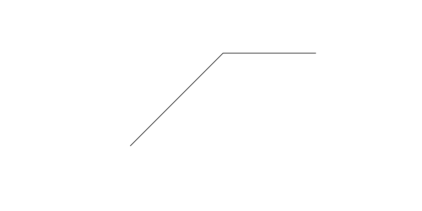
line1 <- st_linestring(x = rbind(c(4,1), c(5,2), c(6,2)))
line1

class(line1)
## [1] "XY"         "LINESTRING" "sfg"

plot(line1)
POLYGON
poly1 <- st_polygon(x = list(rbind(c(1,1), c(3,1), c(3,2), c(1,2), c(.5,.5), c(1,1))))
poly1

class(poly1)
## [1] "XY"      "POLYGON" "sfg"

plot(poly1)

POLYGON (with holes)
poly2 <- st_polygon(x = list(
  # outer polygon
  rbind(c(1,3), c(3,3), c(3,4), c(1,4), c(.5,2.5), c(1,3)),

  # hole1
  rbind(c(1.5, 3.5), c(1.7, 3.5), c(1.7, 3.7), c(1.5, 3.7), c(1.5, 3.5)),

  # hole2
  rbind(c(2.5, 3.5), c(2.7, 3.5), c(2.7, 3.7), c(2.5, 3.5))
))
poly2

class(poly2)
## [1] "XY"      "POLYGON" "sfg"

plot(poly2)

You can also define a Simple Feature Geometry that includes multiple points, linestrings, polygons, or a mixture of all three.
MULTIPOINT
multipt <- st_multipoint(rbind(c(1,1), c(2,2), c(1.5,1.5), c(2,1)))
multipt

class(multipt)
## [1] "XY"         "MULTIPOINT" "sfg"

plot(multipt)

GEOMETRYCOLLECTION (a point, line, and polygon)
geomcoll <- st_geometrycollection(x = list(pt1, line1, poly2))

class(geomcoll)
## [1] "XY"                 "GEOMETRYCOLLECTION" "sfg"

plot(geomcoll)

Notice that printing the objects returns a description of its coordinates. This textual description is called Well Known Text (WKT).
We can do lots of cool things with geometries like
create new point which is pt1 shifted one unit up
pt1 + c(0, 1)
get the area of polygon1
st_area(poly1)
## [1] 2.25
determine if pt1 lies inside poly2
st_within(pt1, poly1, sparse = F)
##       [,1]
## [1,] FALSE
determine the distance between two points
st_distance(st_point(c(1,1)), st_point(c(2,2)))
##          [,1]
## [1,] 1.414214
Simple Feature List-Column (sfc)
Suppose we shoot bullets at a target. We’ll want to analyze where each bullet hit the target. For this we can use a Simple Feature List-Column (sfc). For example
shot1 <- st_point(c(0.4, 0.3))
shot2 <- st_point(c(0.8, 0.1))
shot3 <- st_point(c(0.6, 0.55))
shotsSFC <- st_sfc(shot1, shot2, shot3)
shotsSFC
## Geometry set for 3 features
## geometry type:  POINT
## dimension:      XY
## bbox:           xmin: 0.4 ymin: 0.1 xmax: 0.8 ymax: 0.55
## CRS:            NA

class(shotsSFC)
## [1] "sfc_POINT" "sfc"

plot(shotsSFC)

Now we can do cool stuff like,
get the distance between every pair of bullets
st_distance(shotsSFC)
##           [,1]      [,2]      [,3]
## [1,] 0.0000000 0.4472136 0.3201562
## [2,] 0.4472136 0.0000000 0.4924429
## [3,] 0.3201562 0.4924429 0.0000000
determine the minimum bounding box that contains all points
st_bbox(shotsSFC)
## xmin ymin xmax ymax
## 0.40 0.10 0.80 0.55
You might be wondering why we created a Simple Feature List-Column instead of a MULTIPOINT object. The reason is because MULTIPOINT is meant to represent one “thing” which happens to have multiple points. In this case, we can consider each shot to be a separate “thing”, so it make sense to represent them as multiple POINT objects within a Simple Feature List-Column. To make this more clear, suppose we use a shotgun (which sprays many beads for each shot) instead of a rifle (one bead per shot). Here we’d represent each shot as a MULTIPOINT, but still organize the collection of shots together as a Simple Feature List-Column.
shot1 <- st_multipoint(rbind(c(0.4, 0.3), c(0.45, 0.32), c(0.42, 0.35)))
shot2 <- st_multipoint(rbind(c(0.8, 0.1)))
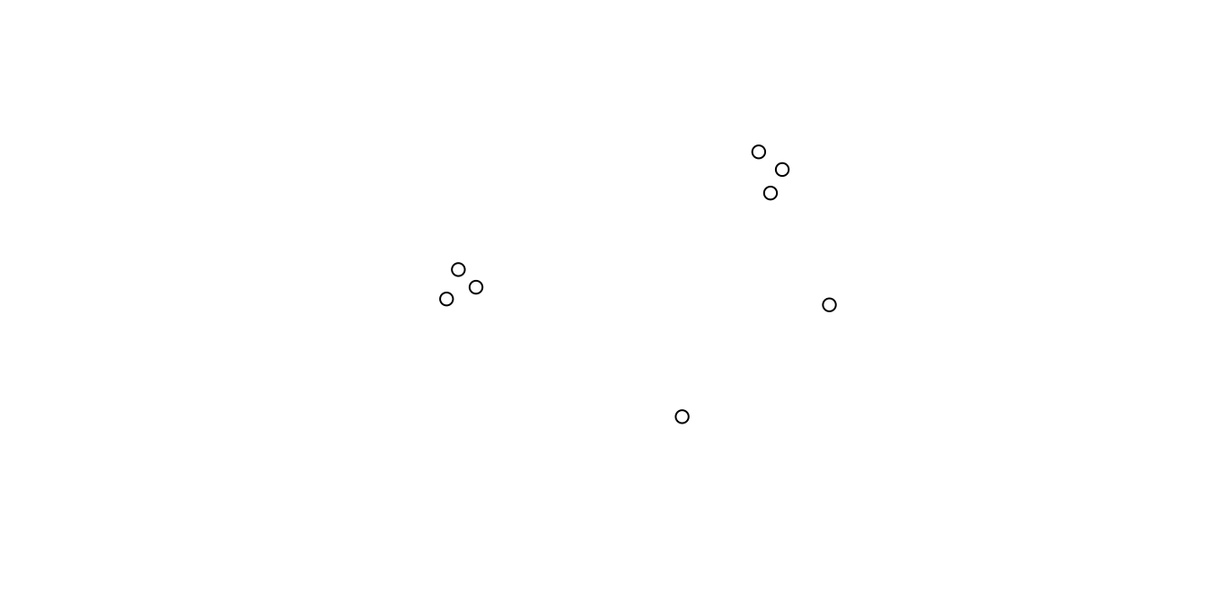
shot3 <- st_multipoint(rbind(c(0.93, 0.55), c(0.97, 0.52), c(0.95, 0.48), c(1.05, 0.29)))
shotsSFC <- st_sfc(shot1, shot2, shot3)
shotsSFC
## Geometry set for 3 features
## geometry type: MULTIPOINT
## dimension: XY
## bbox: xmin: 0.4 ymin: 0.1 xmax: 1.05 ymax: 0.55
## CRS: NA
class(shotsSFC)
## [1] "sfc_MULTIPOINT" "sfc"
plot(shotsSFC)
Simple Feature (sf)
The next layer up from Simple Feature List-Column is the Simple Feature class. Consider our example of shooting a gun at target. With each shot there is associated data we’d like to retain. For example, the shot number and the type of gun used. ShotNumber and GunType are the features associated with the points representing the bullet locations. This concept of having a geometry associated with a set of features is the underlying concept behind the Simple Feature class type.
shotsDF <- data.frame(
  ShotNumber = c(1, 2, 3, 4, 5),
  GunType = c("rifle", "rifle", "shotgun", "shotgun", "shotgun")
)
shot1 <- st_point(c(0.2, 0.75))
shot2 <- st_point(c(1.1, 0.9))
shot3 <- st_multipoint(rbind(c(0.4, 0.3), c(0.45, 0.32), c(0.42, 0.35)))
shot4 <- st_multipoint(rbind(c(0.8, 0.1)))
shot5 <- st_multipoint(rbind(c(0.93, 0.55), c(0.97, 0.52), c(0.95, 0.48), c(1.05, 0.48)))
shotsSFG <- st_sfc(shot1, shot2, shot3, shot4, shot5)
shotsSF <- st_sf(shotsDF, shotsSFG)
shotsSF
## Simple feature collection with 5 features and 2 fields
## geometry type:  GEOMETRY
## dimension:      XY
## bbox:           xmin: 0.2 ymin: 0.1 xmax: 1.1 ymax: 0.9
## CRS:            NA
##   ShotNumber GunType                       shotsSFG
## 1          1   rifle               POINT (0.2 0.75)
## 2          2   rifle                POINT (1.1 0.9)
## 3          3 shotgun MULTIPOINT ((0.4 0.3), (0.4...
## 4          4 shotgun         MULTIPOINT ((0.8 0.1))
## 5          5 shotgun MULTIPOINT ((0.93 0.55), (0...

class(shotsSF)
## [1] "sf"         "data.frame"

plot(shotsSF)
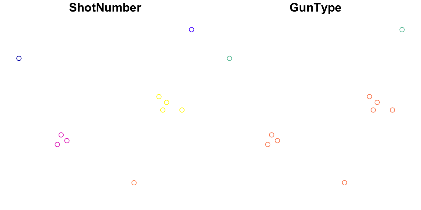
Notice that when we print shotsSF it looks much like a data.frame. In fact, class(shotsSF) returns “sf”, “data.frame” meaning shotsSF is an extension of a data.frame with additional properties defined for Simple Feature objects. The upshot of this is that we can use it much like we use a normal data.frame
subset rows
shotsSF[1:3,]
## Simple feature collection with 3 features and 2 fields
## geometry type:  GEOMETRY
## dimension:      XY
## bbox:           xmin: 0.2 ymin: 0.3 xmax: 1.1 ymax: 0.9
## CRS:            NA
##   ShotNumber GunType                       shotsSFG
## 1          1   rifle               POINT (0.2 0.75)
## 2          2   rifle                POINT (1.1 0.9)
## 3          3 shotgun MULTIPOINT ((0.4 0.3), (0.4...
combine rows
rbind(shotsSF, shotsSF)
## Simple feature collection with 10 features and 2 fields
## geometry type:  GEOMETRY
## dimension:      XY
## bbox:           xmin: 0.2 ymin: 0.1 xmax: 1.1 ymax: 0.9
## CRS:            NA
##    ShotNumber GunType                       shotsSFG
## 1           1   rifle               POINT (0.2 0.75)
## 2           2   rifle                POINT (1.1 0.9)
## 3           3 shotgun MULTIPOINT ((0.4 0.3), (0.4...
## 4           4 shotgun         MULTIPOINT ((0.8 0.1))
## 5           5 shotgun MULTIPOINT ((0.93 0.55), (0...
## 6           1   rifle               POINT (0.2 0.75)
## 7           2   rifle                POINT (1.1 0.9)
## 8           3 shotgun MULTIPOINT ((0.4 0.3), (0.4...
## 9           4 shotgun         MULTIPOINT ((0.8 0.1))
## 10          5 shotgun MULTIPOINT ((0.93 0.55), (0...
reference columns
shotsSF$GunType
## [1] "rifle"   "rifle"   "shotgun" "shotgun" "shotgun"
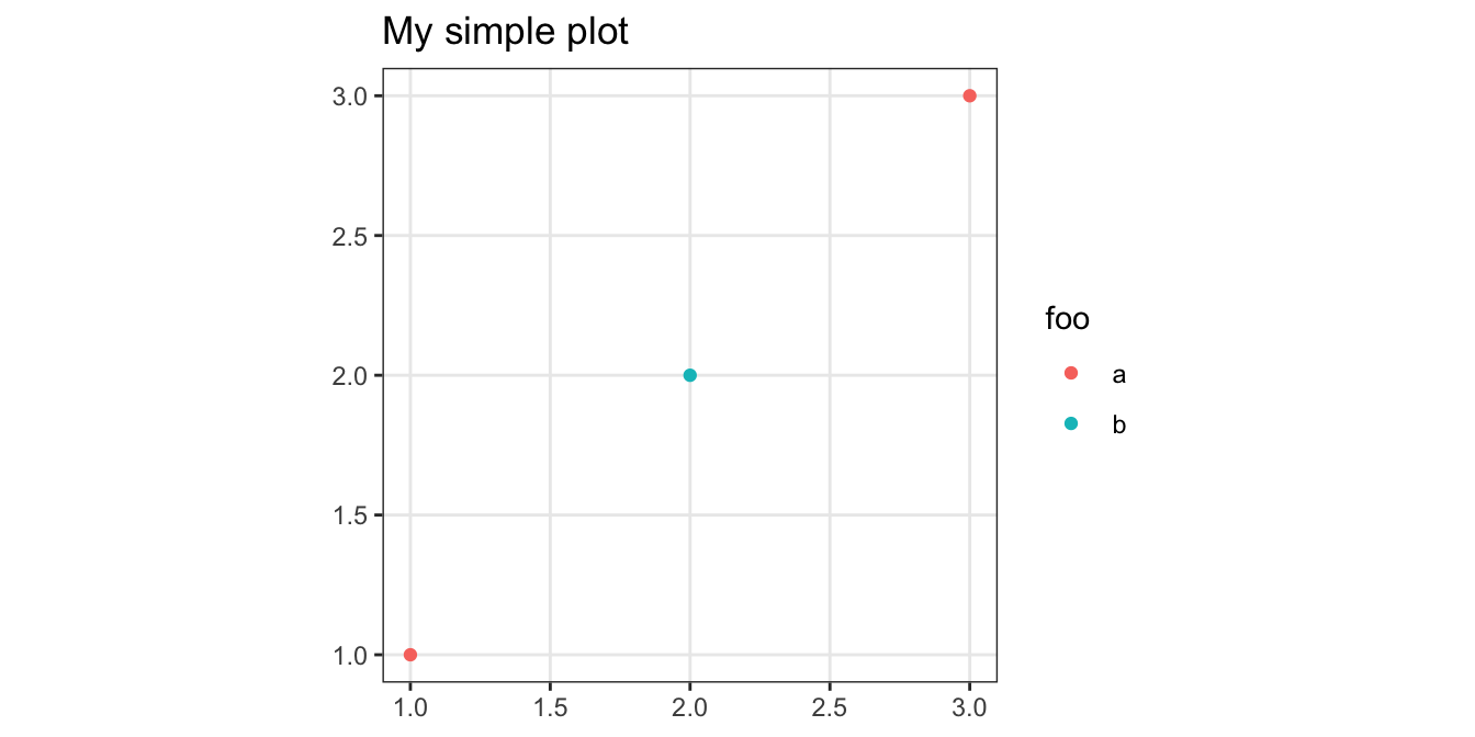
Simple Feature is the class type you’ll use most frequently when working with spatial data. A major benefit to this is that ggplot2 has a native geom_sf() method for plotting your Simple Feature objects. For example
library(ggplot2)

mypoints <- data.frame(x = c(1,2,3), y = c(1,2,3), foo = c("a", "b", "a"))
mypoints <- st_as_sf(mypoints, coords = c("x", "y"))

ggplot()+
  geom_sf(data = mypoints, aes(color = foo))+
  labs(title = "My simple plot")+
  theme_bw()
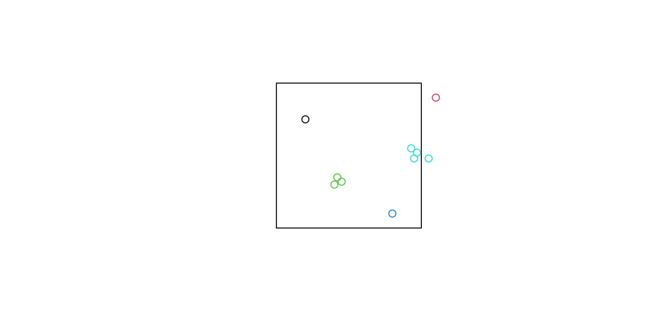
Here we define a square target to illustrate some of the cool things you can do with sf objects.
target <- st_polygon(list(rbind(c(0,0), c(1,0), c(1,1), c(0,1), c(0,0))))

plot(target)
plot(shotsSF, add = T, col = shotsSF$ShotNumber)
Which shots hit the target at least a little bit?
st_intersects(target, shotsSF, sparse = F)
##      [,1]  [,2] [,3] [,4] [,5]
## [1,] TRUE FALSE TRUE TRUE TRUE
Which shots landed entirely within the target?
st_contains(target, shotsSF, sparse = F)
##      [,1]  [,2] [,3] [,4]  [,5]
## [1,] TRUE FALSE TRUE TRUE FALSE
For each shot, how close was the center of the target to the nearest bead?
st_distance(shotsSF, st_centroid(target))
##           [,1]
## [1,] 0.3905125
## [2,] 0.7211103
## [3,] 0.1700000
## [4,] 0.5000000
## [5,] 0.4328972
For each shot, how close was the center of the target to the center of the beads?
st_distance(st_centroid(shotsSF), st_centroid(target))
##           [,1]
## [1,] 0.3905125
## [2,] 0.7211103
## [3,] 0.1925848
## [4,] 0.5000000
## [5,] 0.4750592
Data with a Coordinate Reference System (CRS)
For geospatial data, we can mimmick the concepts above but we’ll need to include something extra – a Coordinate Reference System (CRS). The CRS will inform sf to treat x and y coordinates as longitude and latitude, and help with operations like plotting and measuring the distance between points. CRS is a deep, technical topic and I won’t pretend to be an expert on it. If you’re interested in understanding it better, I’ll defer you to the Wikipedia article for Spatial Reference Systems.
Geospatial data is typically stored as a “shape file” which is really a collection of files that store information about the data. As an example, the sf package comes with a shape file representing the counties in North Carolina. You can see them by navigating to
system.file("shape", package = "sf")  # For me, /Library/Frameworks/R.framework/Versions/3.4/Resources/library/sf/shape
## [1] "/usr/local/Cellar/r/4.0.0/lib/R/library/sf/shape"
list.files(system.file("shape", package = "sf"))
##  [1] "nc.dbf"                  "nc.prj"
##  [3] "nc.shp"                  "nc.shx"
##  [5] "olinda1.dbf"             "olinda1.prj"
##  [7] "olinda1.shp"             "olinda1.shx"
##  [9] "storms_xyz_feature.dbf"  "storms_xyz_feature.shp"
## [11] "storms_xyz_feature.shx"  "storms_xyz.dbf"
## [13] "storms_xyz.shp"          "storms_xyz.shx"
## [15] "storms_xyzm_feature.dbf" "storms_xyzm_feature.shp"
## [17] "storms_xyzm_feature.shx" "storms_xyzm.dbf"
## [19] "storms_xyzm.shp"         "storms_xyzm.shx"
To load a shape file, we can do
nc <- st_read(system.file("shape/nc.shp", package = "sf"))
## Reading layer `nc' from data source `/usr/local/Cellar/r/4.0.0/lib/R/library/sf/shape/nc.shp' using driver `ESRI Shapefile'
## Simple feature collection with 100 features and 14 fields
## geometry type:  MULTIPOLYGON
## dimension:      XY
## bbox:           xmin: -84.32385 ymin: 33.88199 xmax: -75.45698 ymax: 36.58965
## CRS:            4267
nc
## Simple feature collection with 100 features and 14 fields
## geometry type:  MULTIPOLYGON
## dimension:      XY
## bbox:           xmin: -84.32385 ymin: 33.88199 xmax: -75.45698 ymax: 36.58965
## CRS:            4267
## First 10 features:
##     AREA PERIMETER CNTY_ CNTY_ID        NAME  FIPS FIPSNO CRESS_ID BIR74 SID74
## 1  0.114     1.442  1825    1825        Ashe 37009  37009        5  1091     1
## 2  0.061     1.231  1827    1827   Alleghany 37005  37005        3   487     0
## 3  0.143     1.630  1828    1828       Surry 37171  37171       86  3188     5
## 4  0.070     2.968  1831    1831   Currituck 37053  37053       27   508     1
## 5  0.153     2.206  1832    1832 Northampton 37131  37131       66  1421     9
## 6  0.097     1.670  1833    1833    Hertford 37091  37091       46  1452     7
## 7  0.062     1.547  1834    1834      Camden 37029  37029       15   286     0
## 8  0.091     1.284  1835    1835       Gates 37073  37073       37   420     0
## 9  0.118     1.421  1836    1836      Warren 37185  37185       93   968     4
## 10 0.124     1.428  1837    1837      Stokes 37169  37169       85  1612     1
##    NWBIR74 BIR79 SID79 NWBIR79                       geometry
## 1       10  1364     0      19 MULTIPOLYGON (((-81.47276 3...
## 2       10   542     3      12 MULTIPOLYGON (((-81.23989 3...
## 3      208  3616     6     260 MULTIPOLYGON (((-80.45634 3...
## 4      123   830     2     145 MULTIPOLYGON (((-76.00897 3...
## 5     1066  1606     3    1197 MULTIPOLYGON (((-77.21767 3...
## 6      954  1838     5    1237 MULTIPOLYGON (((-76.74506 3...
## 7      115   350     2     139 MULTIPOLYGON (((-76.00897 3...
## 8      254   594     2     371 MULTIPOLYGON (((-76.56251 3...
## 9      748  1190     2     844 MULTIPOLYGON (((-78.30876 3...
## 10     160  2038     5     176 MULTIPOLYGON (((-80.02567 3...
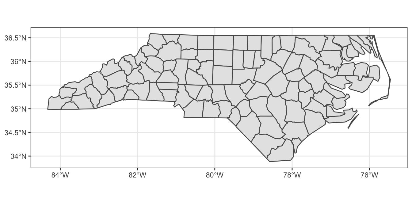
Notice that the resulting object is a Simple Feature where each row in the data.frame represents a county, and the geometry used to represent counties is a MULTIPOLYGON. This is because some counties in NC have disjoint sections broken apart by water.
Heres a plot of the data
ggplot()+geom_sf(data = nc)+theme_bw()
Also take note of the CRS (SRID 4267).
st_crs(nc)
## Coordinate Reference System:
##   User input: 4267
##   wkt:
## GEOGCS["NAD27",
##     DATUM["North_American_Datum_1927",
##         SPHEROID["Clarke 1866",6378206.4,294.9786982138982,
##             AUTHORITY["EPSG","7008"]],
##         AUTHORITY["EPSG","6267"]],
##     PRIMEM["Greenwich",0,
##         AUTHORITY["EPSG","8901"]],
##     UNIT["degree",0.0174532925199433,
##         AUTHORITY["EPSG","9122"]],
##     AUTHORITY["EPSG","4267"]]
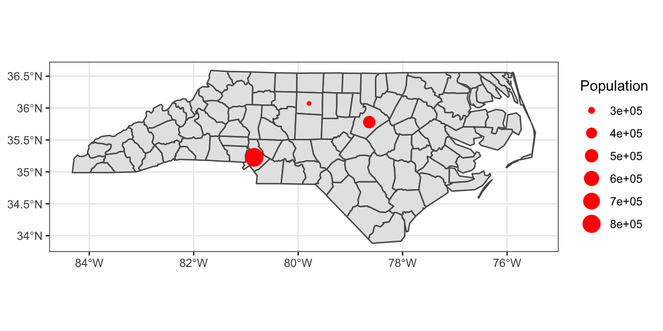
Suppose we want to plot a few cities on the map. First we can build a table of some major cities in NC
cities <- data.frame(
  City = c("Charlotte", "Raleigh", "Greensboro"),
  Population = c(842051, 458880, 287027),
  lon = c(-80.8431, -78.6382, -79.7920),
  lat = c(35.2271, 35.7796, 36.0726)
)
Convert to sf object
citiesSF <- st_as_sf(cities, coords = c("lon", "lat"), crs = 4267)
Plot North Carolina counties with major cities overlaid
ggplot()+
  geom_sf(data = nc)+
  geom_sf(data = citiesSF, aes(size = Population), color = "red")+
  theme_bw()
For more details, be sure to check out the sf vignettes, starting with this one.