Neural Networks – A Worked Example
The purpose of this article is to hold your hand through the process of designing and training a neural network.
Note that this article is Part 2 of Introduction to Neural Networks. R code for this tutorial is provided here in the Machine Learning Problem Bible.
Description of the problem
We start with a motivational problem. We have a collection of 2x2 grayscale images. We’ve identified each image as having a “stairs” like pattern or not. Here’s a subset of those.
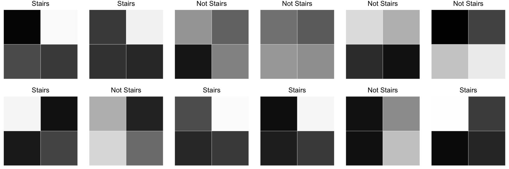
Our goal is to build and train a neural network that can identify whether a new 2x2 image has the stairs pattern.
Description of the network
Our problem is one of binary classification. That means our network could have a single output node that predicts the probability that an incoming image represents stairs. However, we’ll choose to interpret the problem as a multi-class classification problem - one where our output layer has two nodes that represent “probability of stairs” and “probability of something else”. This is unnecessary, but it will give us insight into how we could extend task for more classes. In the future, we may want to classify {“stairs pattern”, “floor pattern”, “ceiling pattern”, or “something else”}.
Our measure of success might be something like accuracy rate, but to implement backpropagation (the fitting procedure) we need to choose a convenient, differentiable loss function like cross entropy. We’ll touch on this more, below.
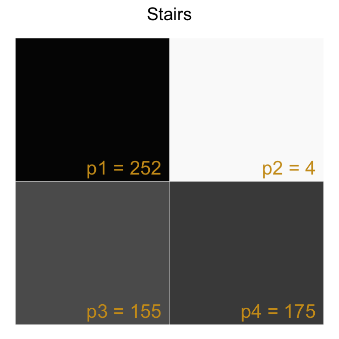
Our training dataset consists of grayscale images. Each image is 2 pixels wide by 2 pixels tall, each pixel representing an intensity between 0 (white) and 255 (black). If we label each pixel intensity as $ p1 $, $ p2 $, $ p3 $, $ p4 $, we can represent each image as a numeric vector which we can feed into our neural network.
| ImageId | p1 | p2 | p3 | p4 | IsStairs |
|---|---|---|---|---|---|
| 1 | 252 | 4 | 155 | 175 | 1 |
| 2 | 175 | 10 | 186 | 200 | 1 |
| 3 | 82 | 131 | 230 | 100 | 0 |
| ... | ... | ... | ... | ... | ... |
| 498 | 36 | 187 | 43 | 249 | 0 |
| 499 | 1 | 160 | 169 | 242 | 1 |
| 500 | 198 | 134 | 22 | 188 | 0 |
For no particular reason, we’ll choose to include one hidden layer with two nodes. We’ll also include bias terms that feed into the hidden layer and bias terms that feed into the output layer. A rough sketch of our network currently looks like this.

Our goal is to find the best weights and biases that fit the training data. To make the optimization process a bit simpler, we’ll treat the bias terms as weights for an additional input node which we’ll fix equal to 1. Now we only have to optimize weights instead of weights and biases. This will reduce the number of objects/matrices we have to keep track of.

Finally, we’ll squash each incoming signal to the hidden layer with a sigmoid function and we’ll squash each incoming signal to the output layer with the softmax function to ensure the predictions for each sample are in the range [0, 1] and sum to 1.

Note here that we’re using the subscript $ i $ to refer to the $ i $th training sample as it gets processed by the network. We use superscripts to denote the layer of the network. And for each weight matrix, the term $ w^l_{ab} $ represents the weight from the $ a $th node in the $ l $th layer to the $ b $th node in the $ (l+1) $th layer. Since keeping track of notation is tricky and critical, we will supplement our algebra with this sample of training data
| ImageId | p1 | p2 | p3 | p4 | IsStairs |
|---|---|---|---|---|---|
| 1 | 252 | 4 | 155 | 175 | 1 |
| 2 | 175 | 10 | 186 | 200 | 1 |
| 3 | 82 | 131 | 230 | 100 | 0 |
| 4 | 115 | 138 | 80 | 88 | 0 |
The matrices that go along with out neural network graph are
$$ \begin{aligned} \mathbf{X^1} &= \begin{bmatrix} x^1_{11} & x^1_{12} & x^1_{13} & x^1_{14} & x^1_{15} \\ x^1_{21} & x^1_{22} & x^1_{23} & x^1_{24} & x^1_{25} \\ … & … & … & … & …\\ x^1_{N1} & x^1_{N2} & x^1_{N3} & x^1_{N4} & x^1_{N5} \end{bmatrix} = \begin{bmatrix} 1 & 252 & 4 & 155 & 175 \\ 1 & 175 & 10 & 186 & 200 \\ 1 & 82 & 131 & 230 & 100 \\ 1 & 115 & 138 & 80 & 88 \end{bmatrix} \\ \mathbf{W^1} &= \begin{bmatrix} w^1_{11} & w^1_{12} \\ w^1_{21} & w^1_{22} \\ w^1_{31} & w^1_{32} \\ w^1_{41} & w^1_{42} \\ w^1_{51} & w^1_{52} \end{bmatrix} \\ \mathbf{Z^1} &= \begin{bmatrix} z^1_{11} & z^1_{12} \\ z^1_{21} & z^1_{22} \\ … & … \\ z^1_{N1} & z^1_{N2} \end{bmatrix} \\ \mathbf{X^2} &= \begin{bmatrix} x^2_{11} & x^2_{12} & x^2_{13} \\ x^2_{21} & x^2_{22} & x^2_{23} \\ … & … & … \\ x^2_{N1} & x^2_{N2} & x^2_{N3} \end{bmatrix} = \begin{bmatrix} 1 & x^2_{12} & x^2_{13} \\ 1 & x^2_{22} & x^2_{23} \\ … & … & … \\ 1 & x^2_{N2} & x^2_{N3} \end{bmatrix} \\ \mathbf{W^2} &= \begin{bmatrix} w^2_{11} & w^2_{12} \\ w^2_{21} & w^2_{22} \\ w^2_{31} & w^2_{32} \end{bmatrix} \\ \mathbf{Z^2} &= \begin{bmatrix} z^2_{11} & z^2_{12} \\ z^2_{21} & z^2_{22} \\ … & … \\ z^2_{N1} & z^2_{N2} \end{bmatrix} \\ \mathbf{Y} &= \begin{bmatrix} y_{11} & y_{12} \\ y_{21} & y_{22} \\ … & … \\ y_{N1} & y_{N2} \end{bmatrix} = \begin{bmatrix} 1 & 0 \\ 1 & 0 \\ 0 & 1 \\ 0 & 1 \end{bmatrix} \\ \widehat{\mathbf{Y}} &= \begin{bmatrix} \widehat{y}{11} & \widehat{y}{12} \\ \widehat{y}{21} & \widehat{y}{22} \\ … & … \\ \widehat{y}{N1} & \widehat{y}{N2} \end{bmatrix} \end{aligned} $$
Initializing the weights
Before we can start the gradient descent process that finds the best weights, we need to initialize the network with random weights. In this case, we’ll pick uniform random values between -0.01 and 0.01.
$$ \begin{aligned} \mathbf{W^1} &= \begin{bmatrix} w^1_{11} & w^1_{12} \\ w^1_{21} & w^1_{22} \\ w^1_{31} & w^1_{32} \\ w^1_{41} & w^1_{42} \\ w^1_{51} & w^1_{52} \end{bmatrix} = \begin{bmatrix} -0.00469 & 0.00797 \\ -0.00256 & 0.00889 \\ 0.00146 & 0.00322 \\ 0.00816 & 0.00258 \\ -0.00597 &-0.00876 \end{bmatrix} \\ \mathbf{W^2} &= \begin{bmatrix} w^2_{11} & w^2_{12} \\ w^2_{21} & w^2_{22} \\ w^2_{31} & w^2_{32} \end{bmatrix} = \begin{bmatrix} -0.00588 & -0.00232 \\ -0.00647 & 0.00540 \\ 0.00374 & -0.00005 \end{bmatrix} \end{aligned} $$
Is it possible to choose bad weights? Yes. Numeric stability often becomes an issue for neural networks and choosing bad weights can exacerbate the problem. There are methods of choosing good initial weights, but that is beyond the scope of this article. (See this for more details.)
Forward Pass
Now let’s walk through the forward pass to generate predictions for each of our training samples.
1. Determine $ \mathbf{Z^1} $
Compute the signal going into the hidden layer, $ \mathbf{Z^1} $
$$ \mathbf{Z^1} = \mathbf{X^1} \mathbf{W^1} $$
$$ \begin{bmatrix} z^1_{11} & z^1_{12} \\ z^1_{21} & z^1_{22} \\ … & … \\ z^1_{N1} & z^1_{N2} \end{bmatrix} = \begin{bmatrix} x^1_{11} & x^1_{12} & x^1_{13} & x^1_{14} & x^1_{15} \\ x^1_{21} & x^1_{22} & x^1_{23} & x^1_{24} & x^1_{25} \\ … & … & … & … & … \\ x^1_{N1} & x^1_{N2} & x^1_{N3} & x^1_{N4} & x^1_{N5} \end{bmatrix} \times \begin{bmatrix} w^1_{11} & w^1_{12} \\ w^1_{21} & w^1_{22} \\ w^1_{31} & w^1_{32} \\ w^1_{41} & w^1_{42} \\ w^1_{51} & w^1_{52} \end{bmatrix} \\ = \begin{bmatrix} x^1_{11}w^1_{11} + x^1_{12}w^1_{21} + … + x^1_{15}w^1_{51} & x^1_{11}w^1_{12} + x^1_{12}w^1_{22} + … + x^1_{15}w^1_{52} \\ x^1_{21}w^1_{11} + x^1_{22}w^1_{21} + … + x^1_{25}w^1_{51} & x^1_{21}w^1_{12} + x^1_{22}w^1_{22} + … + x^1_{25}w^1_{52} \\ … & … \\ x^1_{N1}w^1_{11} + x^1_{N2}w^1_{21} + … + x^1_{N5}w^1_{51} & x^1_{N1}w^1_{12} + x^1_{N2}w^1_{22} + … + x^1_{N5}w^1_{52} \end{bmatrix} $$
2. Determine $ \mathbf{X^2} $
Squash the signal to the hidden layer with the sigmoid function to determine the inputs to the output layer, $ \mathbf{X^2} $
$$ sigmoid(z) = 1/(1 + e^{-z}) $$
$$ \mathbf{X^2} = \begin{bmatrix} \mathbf{1} & sigmoid(\mathbf{Z^1}) \end{bmatrix} $$
$$ \begin{bmatrix} x^2_{11} & x^2_{12} & x^2_{13} \\ x^2_{21} & x^2_{22} & x^2_{23} \\ … & … & … \\ x^2_{N1} & x^2_{N2} & x^2_{N3} \end{bmatrix} = \begin{bmatrix} 1 & sigmoid(z^1_{11}) & sigmoid(z^1_{12}) \\ 1 & sigmoid(z^1_{21}) & sigmoid(z^1_{22}) \\ … & … & … \\ 1 & sigmoid(z^1_{N1}) & sigmoid(z^1_{N2}) \end{bmatrix} = \begin{bmatrix} 1 & \frac{1}{1 + e^{-z^1_{11}}} & \frac{1}{1 + e^{-z^1_{12}}} \\ 1 & \frac{1}{1 + e^{-z^1_{21}}} & \frac{1}{1 + e^{-z^1_{22}}} \\ … & … & … \\ 1 & \frac{1}{1 + e^{-z^1_{N1}}} & \frac{1}{1 + e^{-z^1_{N2}}} \end{bmatrix} $$
3. Determine $ \mathbf{Z^2} $
Calculate the signal going into the output layer, $ \mathbf{Z^2} $
$$ \mathbf{Z^2} = \mathbf{X^2}\mathbf{W^2} $$
$$ \begin{bmatrix} z^2_{11} & z^2_{12} \\ z^2_{21} & z^2_{22} \\ … & … \\ z^2_{N1} & z^2_{N2} \end{bmatrix} = \begin{bmatrix} x^2_{11} & x^2_{12} & x^2_{13} \\ x^2_{21} & x^2_{22} & x^2_{23} \\ … & … & … \\ x^2_{N1} & x^2_{N2} & x^2_{N3} \end{bmatrix} \times \begin{bmatrix} w^2_{11} & w^2_{12} \\ w^2_{21} & w^2_{22} \\ w^2_{31} & w^2_{32} \end{bmatrix} = \\ \begin{bmatrix} x^2_{11}w^2_{11} + x^2_{12}w^2_{21} + x^2_{13}w^2_{31} & x^2_{11}w^2_{12} + x^2_{12}w^2_{22} + x^2_{13}w^2_{32} \\ x^2_{21}w^2_{11} + x^2_{22}w^2_{21} + x^2_{23}w^2_{31} & x^2_{21}w^2_{12} + x^2_{22}w^2_{22} + x^2_{23}w^2_{32} \\ … & … \\ x^2_{N1}w^2_{11} + x^2_{N2}w^2_{21} + x^2_{N3}w^2_{31} & x^2_{N1}w^2_{12} + x^2_{N2}w^2_{22} + x^2_{N3}w^2_{32} \end{bmatrix} $$
4. Determine $ \widehat{\mathbf{Y}} $
Squash the signal to the output layer with the softmax function to determine the predictions, $ \widehat{\mathbf{Y}} $. Recall that the softmax function is a mapping from $ \mathbb{R}^n $ to $ \mathbb{R}^n $. In other words, it takes a vector $ \theta $ as input and returns an equal size vector as output. For the $ k $th element of the output,
$$ softmax(\theta)_k = \frac{e^{\theta_k}}{ \sum_{j=1}^n e^{\theta_j} } $$
In our model, we apply the softmax function to each vector of predicted probabilities. In other words, we apply the softmax function “row-wise” to $ \mathbf{Z^2} $.
$$ \widehat{\mathbf{Y}} = softmax_{row-wise}(\mathbf{Z^2}) $$
$$ \begin{aligned} \begin{bmatrix} \widehat{y}_{11} & \widehat{y}_{12} \\ \widehat{y}_{21} & \widehat{y}_{22} \\ … & … \\ \widehat{y}_{N1} & \widehat{y}_{N2} \end{bmatrix} &= \begin{bmatrix} softmax(\begin{bmatrix} z^2_{11} & z^2_{12}) \end{bmatrix})1 & softmax(\begin{bmatrix} z^2{11} & z^2_{12}) \end{bmatrix})2 \\ softmax(\begin{bmatrix} z^2{21} & z^2_{22}) \end{bmatrix})1 & softmax(\begin{bmatrix} z^2{21} & z^2_{22}) \end{bmatrix})2 \\ … & … \\ softmax(\begin{bmatrix} z^2{N1} & z^2_{N2}) \end{bmatrix})1 & softmax(\begin{bmatrix} z^2{N1} & z^2_{N2}) \end{bmatrix})2 \end{bmatrix} \\ &= \begin{bmatrix} e^{z^2{11}}/(e^{z^2_{11}} + e^{z^2_{12}}) & e^{z^2_{12}}/(e^{z^2_{11}} + e^{z^2_{12}}) \\ e^{z^2_{21}}/(e^{z^2_{21}} + e^{z^2_{22}}) & e^{z^2_{22}}/(e^{z^2_{21}} + e^{z^2_{22}}) \\ … & … \\ e^{z^2_{N1}}/(e^{z^2_{N1}} + e^{z^2_{N2}}) & e^{z^2_{N2}}/(e^{z^2_{N1}} + e^{z^2_{N2}}) \end{bmatrix} \end{aligned} $$
Running the forward pass on our sample data gives
$$ \mathbf{Z^1} = \begin{bmatrix} -0.42392 & 1.12803 \\ -0.11433 & 0.32380 \\ 1.25645 & 0.87617 \\ 0.02983 & 0.91020 \end{bmatrix}, \mathbf{X^2} = \begin{bmatrix} 1 & 0.39558 & 0.75548 \\ 1 & 0.47145 & 0.58025 \\ 1 & 0.77841 & 0.70603 \\ 1 & 0.50746 & 0.71304 \end{bmatrix} $$
$$ \mathbf{Z^2} = \begin{bmatrix} -0.00561 & -0.00022 \\ -0.00676 & 0.00020 \\ -0.00828 & 0.00185 \\ -0.00650 & 0.00038 \end{bmatrix}, \widehat{\mathbf{Y}} = \begin{bmatrix} 0.49865 & 0.50135 \\ 0.49826 & 0.50174 \\ 0.49747 & 0.50253 \\ 0.49828 & 0.50172 \end{bmatrix} $$
Backpropagation
Our strategy to find the optimal weights is gradient descent. Since we have a set of initial predictions for the training samples we’ll start by measuring the model’s current performance using our loss function, cross entropy. The loss associated with the $ i $th prediction would be
$$ CE_i = CE(\widehat{\mathbf Y_{i,}} \mathbf Y_{i,}) = -\sum_{c = 1}^{C} y_{ic} \log (\widehat{y}_{ic}) $$
where $ c $ iterates over the target classes.
Note here that $ CE $ is only affected by the prediction value associated with the True instance. For example, if we were doing a 3-class prediction problem and $ y $ = [0, 1, 0], then $ \widehat y $ = [0, 0.5, 0.5] and $ \widehat y $ = [0.25, 0.5, 0.25] would both have $ CE = 0.69 $.
The cross entropy loss of our entire training dataset would then be the average $ CE_i $ over all samples. For our training data, after our initial forward pass we’d have
| ImageId | x1 | x2 | x3 | x4 | IsStairs | Yhat_Stairs | Yhat_Else | CE |
|---|---|---|---|---|---|---|---|---|
| 1 | 252 | 4 | 155 | 175 | TRUE | 0.4986519 | 0.5013481 | 0.6958470 |
| 2 | 175 | 10 | 186 | 200 | TRUE | 0.4982608 | 0.5017392 | 0.6966317 |
| 3 | 82 | 131 | 230 | 100 | FALSE | 0.4974690 | 0.5025310 | 0.6880980 |
| 4 | 115 | 138 | 80 | 88 | FALSE | 0.4982797 | 0.5017203 | 0.6897126 |
$$ CE = 0.69257 $$
Next, we need to determine how a “small” change in each of the weights would affect our current loss. In other words, we want to determine $ \frac{\partial CE}{\partial w^1_{11}} $, $ \frac{\partial CE}{\partial w^1_{12}} $, … $ \frac{\partial CE}{\partial w^2_{32}} $ which is the gradient of $ CE $ with respect to each of the weight matrices, $ \nabla_{\mathbf{W^1}}CE $ and $ \nabla_{\mathbf{W^2}}CE $.
To start, recognize that $ \frac{\partial CE}{\partial w_{ab}} = \frac{1}{N} \left[ \frac{\partial CE_1}{\partial w_{ab}} + \frac{\partial CE_2}{\partial w_{ab}} + … \frac{\partial CE_N}{\partial w_{ab}} \right] $ where $ \frac{\partial CE_i}{\partial w_{ab}} $ is the rate of change of [$ CE$ of the $ i $th sample] with respect to weight $ w_{ab} $. In light of this, let’s concentrate on calculating $ \frac{\partial CE_1}{w_{ab}} $, “How much will $ CE $ of the first training sample change with respect to a small change in $ w_{ab} $?”. If we can calculate this, we can calculate $ \frac{\partial CE_2}{\partial w_{ab}} $ and so forth, and then average the partials to determine the overall expected change in $ CE $ with respect to a small change in $ w_{ab} $.
Recall our network diagram.
1. Determine $ \frac{\partial CE_1}{\partial \widehat{\mathbf{Y_{1,}}}} $
$$ \frac{\partial CE_1}{\widehat{\mathbf{Y_{1,}}}} = \begin{bmatrix} \frac{\partial CE_1}{\widehat y_{11}} & \frac{\partial CE_1}{\widehat y_{12}} \end{bmatrix} $$
Recall $ CE_1 = CE(\widehat{\mathbf Y_{1,}}, \mathbf Y_{1,}) = -(y_{11}\log{\widehat y_{11}} + y_{12}\log{\widehat y_{12}}) $
So
$$ \frac{\partial CE_1}{\partial \widehat{\mathbf{Y_{1,}}}} = \begin{bmatrix} \frac{-y_{11}}{\widehat y_{11}} & \frac{-y_{12}}{\widehat y_{12}} \end{bmatrix} $$
2. Determine $ \frac{\partial CE_1}{\partial \mathbf{Z^2_{1,}}} $
$$ \def \matONE{ \begin{bmatrix} \frac{\partial CE_1}{\partial z^2_{11}} & \frac{\partial CE_1}{\partial z^2_{12}} \end{bmatrix} } \def \matTWO{ \begin{bmatrix} \frac{\partial CE_1}{\partial \widehat y_{11}} \frac{\partial \widehat y_{11}}{\partial z^2_{11}} + \frac{\partial CE_1}{\partial \widehat y_{12}} \frac{\partial \widehat y_{12}}{\partial z^2_{11}} & \frac{\partial CE_1}{\partial \widehat y_{11}} \frac{\partial \widehat y_{11}}{\partial z^2_{12}} + \frac{\partial CE_1}{\partial \widehat y_{12}} \frac{\partial \widehat y_{12}}{\partial z^2_{12}} \end{bmatrix} } \def \matTHREE{ \begin{bmatrix} \frac{\partial CE_1}{\partial \widehat y_{11}} & \frac{\partial CE_1}{\partial \widehat y_{12}} \end{bmatrix} } \def \matFOUR{ \begin{bmatrix} \frac{\partial \widehat y_{11}}{\partial z^2_{11}} & \frac{\partial \widehat y_{11}}{\partial z^2_{12}} \\ \frac{\partial \widehat y_{12}}{\partial z^2_{11}} & \frac{\partial \widehat y_{12}}{\partial z^2_{12}} \end{bmatrix} } \begin{aligned} \frac{\partial CE_1}{\partial \mathbf{Z^2_{1,}}} &= \matONE \\ &= \matTWO \\ &= \matTHREE \times \matFOUR \\ &= \frac{\partial CE_1}{\partial \widehat{\mathbf{Y_{1,}}}} \frac{\partial \widehat{\mathbf{Y_{1,}}}}{\partial \mathbf{Z^2_{1,}}} \end{aligned} $$
We need to determine expressions for the elements of
$$ \frac{\partial \widehat{\mathbf{Y_{1,}}}}{\partial \mathbf{Z^2_{1,}}} = \begin{bmatrix} \frac{\partial \widehat y_{11}}{\partial z^2_{11}} & \frac{\partial \widehat y_{11}}{\partial z^2_{12}} \\ \frac{\partial \widehat y_{12}}{\partial z^2_{11}} & \frac{\partial \widehat y_{12}}{\partial z^2_{12}} \end{bmatrix} $$
Recall
$$ \widehat{\mathbf{Y_{1,}}} = \begin{bmatrix} \widehat y_{11} & \widehat y_{12} \end{bmatrix} = softmax(\begin{bmatrix} z^2_{11} & z^2_{12} \end{bmatrix}) = \begin{bmatrix} \frac{e^{z^2_{11}}}{e^{z^2_{11}} + e^{z^2_{12}}} & \frac{e^{z^2_{12}}}{e^{z^2_{11}} + e^{z^2_{12}}} \end{bmatrix} $$
We can make use of the quotient rule to show
$$ \frac{\partial softmax(\theta)_c}{\partial \theta_j} = {\begin{cases} (softmax(\theta)_c)(1 - softmax(\theta)_c)&{\text{if }} j = c \\ (-softmax(\theta)_c)(softmax(\theta)_j)&{\text{otherwise}} \end{cases}} $$
Hence,
$$ \frac{\partial \widehat{\mathbf{Y_{1,}}}}{\partial \mathbf{Z^2_{1,}}} = \begin{bmatrix} \frac{\partial \widehat y_{11}}{\partial z^2_{11}} = \widehat y_{11}(1 - \widehat y_{11}) & \frac{\partial \widehat y_{11}}{\partial z^2_{12}} = -\widehat y_{12}\widehat y_{11} \\ \frac{\partial \widehat y_{12}}{\partial z^2_{11}} = -\widehat y_{11}\widehat y_{12} & \frac{\partial \widehat y_{12}}{\partial z^2_{12}} = \widehat y_{12}(1 - \widehat y_{12}) \end{bmatrix} $$
Now we have
$$ \def \matONE{ \begin{bmatrix} \frac{-y_{11}}{\widehat y_{11}} & \frac{-y_{12}}{\widehat y_{12}} \end{bmatrix} } \def \matTWO{ \begin{bmatrix} \widehat y_{11}(1 - \widehat y_{11}) & -\widehat y_{12}\widehat y_{11} \\ -\widehat y_{11}\widehat y_{12} & \widehat y_{12}(1 - \widehat y_{12}) \end{bmatrix} } \def \matTHREE{ \begin{bmatrix} -y_{11}(1 - \widehat y_{11}) + y_{12} \widehat y_{11} & y_{11} \widehat y_{12} - y_{12} (1 - \widehat y_{12}) \end{bmatrix} } \def \matFOUR{ \begin{bmatrix} \widehat y_{11} - y_{11} & \widehat y_{12} - y_{12} \end{bmatrix} } \begin{aligned} \frac{\partial CE_1}{\partial \widehat{\mathbf{Y_{1,}}}} \frac{\partial \widehat{\mathbf{Y_{1,}}}}{\partial \mathbf{Z^2_{1,}}} &= \matONE \times \matTWO \\ &= \matTHREE \\ &= \matFOUR \\ &= \widehat{\mathbf{Y_{1,}}} - \mathbf{Y_{1,}} \end{aligned} $$
3. Determine $ \frac{\partial CE_1}{\partial \mathbf{W^2}} $
$$ \def \matONE{ \begin{bmatrix} \frac{\partial CE_1}{\partial w^2_{11}} & \frac{\partial CE_1}{\partial w^2_{12}} \\ \frac{\partial CE_1}{\partial w^2_{21}} & \frac{\partial CE_1}{\partial w^2_{22}} \\ \frac{\partial CE_1}{\partial w^2_{31}} & \frac{\partial CE_1}{\partial w^2_{32}} \end{bmatrix} } \def \matTWO{ \begin{bmatrix} \frac{\partial CE_1}{\partial z^2_{11}} \frac{\partial z^2_{11}}{\partial w^2_{11}} & \frac{\partial CE_1}{\partial z^2_{12}} \frac{\partial z^2_{12}}{\partial w^2_{12}} \\ \frac{\partial CE_1}{\partial z^2_{11}} \frac{\partial z^2_{11}}{\partial w^2_{21}} & \frac{\partial CE_1}{\partial z^2_{12}} \frac{\partial z^2_{12}}{\partial w^2_{22}} \\ \frac{\partial CE_1}{\partial z^2_{11}} \frac{\partial z^2_{11}}{\partial w^2_{31}} & \frac{\partial CE_1}{\partial z^2_{12}} \frac{\partial z^2_{12}}{\partial w^2_{32}} \end{bmatrix} } \def \matTHREE{ \begin{bmatrix} \frac{\partial CE_1}{\partial z^2_{11}} x^2_{11} & \frac{\partial CE_1}{\partial z^2_{12}} x^2_{11} \\ \frac{\partial CE_1}{\partial z^2_{11}} x^2_{12} & \frac{\partial CE_1}{\partial z^2_{12}} x^2_{12} \\ \frac{\partial CE_1}{\partial z^2_{11}} x^2_{13} & \frac{\partial CE_1}{\partial z^2_{12}} x^2_{13} \end{bmatrix} } \def \matFOUR{ \begin{bmatrix} x^2_{11} \\ x^2_{12} \\ x^2_{13} \end{bmatrix} } \def \matFIVE{ \begin{bmatrix} \frac{\partial CE_1}{\partial z^2_{11}} & \frac{\partial CE_1}{\partial z^2_{12}} \end{bmatrix} } \begin{aligned} \frac{\partial CE_1}{\partial \mathbf{W^2}} &= \matONE \\ &= \matTWO \\ &= \matTHREE \\ &= \matFOUR \times \matFIVE \\ &= (\mathbf{X^2_{1,}})^T(\widehat{\mathbf{Y_{1,}}} - \mathbf{Y_{1,}}) \end{aligned} $$
4. Determine $ \frac{\partial CE_1}{\partial \mathbf{X^2_{1,}}} $
$$ \def \matONE{ \begin{bmatrix} \frac{\partial CE_1}{\partial x^2_{11}} & \frac{\partial CE_1}{\partial x^2_{12}} & \frac{\partial CE_1}{\partial x^2_{13}} \end{bmatrix} } \def \matTWO{ \begin{bmatrix} \frac{\partial CE_1}{\partial z^2_{11}} \frac{\partial z^2_{11}}{\partial x^2_{11}} + \frac{\partial CE_1}{\partial z^2_{12}} \frac{\partial z^2_{12}}{\partial x^2_{11}} & \frac{\partial CE_1}{\partial z^2_{11}} \frac{\partial z^2_{11}}{\partial x^2_{12}} + \frac{\partial CE_1}{\partial z^2_{12}} \frac{\partial z^2_{12}}{\partial x^2_{12}} & \frac{\partial CE_1}{\partial z^2_{11}} \frac{\partial z^2_{11}}{\partial x^2_{13}} + \frac{\partial CE_1}{\partial z^2_{12}} \frac{\partial z^2_{12}}{\partial x^2_{13}} \end{bmatrix} } \def \matTHREE{ \begin{bmatrix} \frac{\partial CE_1}{\partial z^2_{11}} w^2_{11} + \frac{\partial CE_1}{\partial z^2_{12}} w^2_{12} & \frac{\partial CE_1}{\partial z^2_{11}} w^2_{21} + \frac{\partial CE_1}{\partial z^2_{12}} w^2_{22} & \frac{\partial CE_1}{\partial z^2_{11}} w^2_{31} + \frac{\partial CE_1}{\partial z^2_{12}} w^2_{32} \end{bmatrix} } \def \matFOUR{ \begin{bmatrix} \frac{\partial CE_1}{\partial z^2_{11}} & \frac{\partial CE_1}{\partial z^2_{12}} \end{bmatrix} } \def \matFIVE{ \begin{bmatrix} w^2_{11} & w^2_{21} & w^2_{31} \\ w^2_{12} & w^2_{22} & w^2_{32} \end{bmatrix} } \begin{aligned} \frac{\partial CE_1}{\partial \mathbf{X^2_{1,}}} &= \matONE \\ &= \matTWO \\ &= \matTHREE \\ &= \matFOUR \times \matFIVE \\ &= \left(\frac{\partial CE_1}{\partial \mathbf{Z^2_{1,}}}\right)\left(\mathbf{W^2}\right)^T \end{aligned} $$
5. Determine $ \frac{\partial CE_1}{\partial \mathbf{Z^1_{1,}}} $
$$ \def \matONE{ \begin{bmatrix} \frac{\partial CE_1}{\partial z^1_{11}} & \frac{\partial CE_1}{\partial z^1_{12}}\end{bmatrix} } \def \matTWO{ \begin{bmatrix} \frac{\partial CE_1}{\partial x^2_{12}} \frac{\partial x^2_{12}}{\partial z^1_{11}} & \frac{\partial CE_1}{\partial x^2_{13}} \frac{\partial x^2_{13}}{\partial z^1_{12}} \end{bmatrix} } \def \matTHREE{ \begin{bmatrix} \frac{\partial CE_1}{\partial x^2_{12}} & \frac{\partial CE_1}{\partial x^2_{13}} \end{bmatrix} } \def \matFOUR{ \begin{bmatrix} \frac{\partial x^2_{12}}{\partial z^1_{11}} & \frac{\partial x^2_{13}}{\partial z^1_{12}} \end{bmatrix} } \def \matFIVE{ \begin{bmatrix} \frac{\partial sigmoid(z^1_{11})}{\partial z^1_{11}} & \frac{\partial sigmoid(z^1_{12})}{\partial z^1_{12}} \end{bmatrix} } \begin{aligned} \frac{\partial CE_1}{\partial \mathbf{Z^1_{1,}}} &= \matONE \\ &= \matTWO \\ &= \matTHREE \otimes \matFOUR \\ &= \matTHREE \otimes \matFIVE \end{aligned} $$
Where $ \otimes $ is the tensor product that does “element-wise” multiplication between matrices.
Next we’ll use the fact that $ \frac{d \, sigmoid(z)}{dz} = sigmoid(z)(1-sigmoid(z)) $ to deduce that the expression above is equivalent to
$$ \def \matONE{ \begin{bmatrix} \frac{\partial CE_1}{\partial x^2_{12}} & \frac{\partial CE_1}{\partial x^2_{13}} \end{bmatrix} } \def \matTWO{ \begin{bmatrix} x^2_{12}(1 - x^2_{12}) & x^2_{13}(1 - x^2_{13}) \end{bmatrix} } \matONE \otimes \matTWO = \frac{\partial CE_1}{\partial \mathbf{X^2_{1,2:}}} \otimes \left( \mathbf{X^2_{1,2:}} \otimes \left( 1 - \mathbf{X^2_{1,2:}} \right) \right) $$
6. Determine $ \frac{\partial CE_1}{\partial \mathbf{W^1}} $
$$ \def \matONE{ \begin{bmatrix} \frac{\partial CE_1}{\partial w^1_{11}} & \frac{\partial CE_1}{\partial w^1_{12}} \\ \frac{\partial CE_1}{\partial w^1_{21}} & \frac{\partial CE_1}{\partial w^1_{22}} \\ \frac{\partial CE_1}{\partial w^1_{31}} & \frac{\partial CE_1}{\partial w^1_{32}} \\ \frac{\partial CE_1}{\partial w^1_{41}} & \frac{\partial CE_1}{\partial w^1_{42}} \\ \frac{\partial CE_1}{\partial w^1_{51}} & \frac{\partial CE_1}{\partial w^1_{52}} \end{bmatrix} } \def \matTWO{ \begin{bmatrix} \frac{\partial CE_1}{\partial z^1_{11}} \frac{\partial z^1_{11}}{\partial w^1_{11}} & \frac{\partial CE_1}{\partial z^1_{12}} \frac{\partial z^1_{12}}{\partial w^1_{12}} \\ \frac{\partial CE_1}{\partial z^1_{11}} \frac{\partial z^1_{11}}{\partial w^1_{21}} & \frac{\partial CE_1}{\partial z^1_{12}} \frac{\partial z^1_{12}}{\partial w^1_{22}} \\ \frac{\partial CE_1}{\partial z^1_{11}} \frac{\partial z^1_{11}}{\partial w^1_{31}} & \frac{\partial CE_1}{\partial z^1_{12}} \frac{\partial z^1_{12}}{\partial w^1_{32}} \\ \frac{\partial CE_1}{\partial z^1_{11}} \frac{\partial z^1_{11}}{\partial w^1_{41}} & \frac{\partial CE_1}{\partial z^1_{12}} \frac{\partial z^1_{12}}{\partial w^1_{42}} \\ \frac{\partial CE_1}{\partial z^1_{11}} \frac{\partial z^1_{11}}{\partial w^1_{51}} & \frac{\partial CE_1}{\partial z^1_{12}} \frac{\partial z^1_{12}}{\partial w^1_{52}} \end{bmatrix} } \def \matTHREE{ \begin{bmatrix} \frac{\partial CE_1}{\partial z^1_{11}} x^1_{11} & \frac{\partial CE_1}{\partial z^1_{12}} x^1_{11} \\ \frac{\partial CE_1}{\partial z^1_{11}} x^1_{12} & \frac{\partial CE_1}{\partial z^1_{12}} x^1_{12} \\ \frac{\partial CE_1}{\partial z^1_{11}} x^1_{13} & \frac{\partial CE_1}{\partial z^1_{12}} x^1_{13} \\ \frac{\partial CE_1}{\partial z^1_{11}} x^1_{14} & \frac{\partial CE_1}{\partial z^1_{12}} x^1_{14} \\ \frac{\partial CE_1}{\partial z^1_{11}} x^1_{15} & \frac{\partial CE_1}{\partial z^1_{12}} x^1_{15} \end{bmatrix} } \def \matFOUR{ \begin{bmatrix} x^1_{11} \\ x^1_{12} \\ x^1_{13} \\ x^1_{14} \\ x^1_{15} \end{bmatrix} } \def \matFIVE{ \begin{bmatrix} \frac{\partial CE_1}{\partial z^1_{11}} & \frac{\partial CE_1}{\partial z^1_{12}} \end{bmatrix} } \begin{aligned} \frac{\partial CE_1}{\partial \mathbf{W^1}} &= \matONE \\ &= \matTWO \\ &= \matTHREE \\ &= \matFOUR \times \matFIVE \\ &= \left(\mathbf{X^1_{1,}}\right)^T \left(\frac{\partial CE_1}{\partial \mathbf{Z^1_{1,}}}\right) \end{aligned} $$
Recap
We have
$$ \begin{aligned} \frac{\partial CE_1}{\partial \mathbf{Z^2_{1,}}} &= \widehat{\mathbf{Y_{1,}}} - \mathbf{Y_{1,}} \\ \frac{\partial CE_1}{\partial \mathbf{X^2_{1,}}} &= \left(\frac{\partial CE_1}{\partial \mathbf{Z^2_{1,}}}\right) \left(\mathbf{W^2}\right)^T \\ \frac{\partial CE_1}{\partial \mathbf{Z^1_{1,}}} &= \frac{\partial CE_1}{\partial \mathbf{X^2_{1,2:}}} \otimes \left( \mathbf{X^2_{1,2:}} \otimes \left( 1 - \mathbf{X^2_{1,2:}} \right) \right) \end{aligned} $$
$$ \boxed{ \frac{\partial CE_1}{\partial \mathbf{W^2}} = \left(\mathbf{X^2_{1,}}\right)^T \left(\frac{\partial CE_1}{\partial \mathbf{Z^2_{1,}}}\right) } \\ \boxed{ \frac{\partial CE_1}{\partial \mathbf{W^1}} = \left(\mathbf{X^1_{1,}}\right)^T \left(\frac{\partial CE_1}{\partial \mathbf{Z^1_{1,}}}\right) } $$
Now we have expressions that we can easily use to compute how cross entropy of the first training sample should change with respect to a small change in each of the weights. These formulas easily generalize to let us compute the change in cross entropy for every training sample as follows.
$$ \begin{aligned} \nabla_{\mathbf{Z^2}}CE &= \widehat{\mathbf{Y}} - \mathbf{Y} \\ \nabla_{\mathbf{X^2}}CE &= \left(\nabla_{\mathbf{Z^2}}CE\right) \left(\mathbf{W^2}\right)^T \\ \nabla_{\mathbf{Z^1}}CE &= \left(\nabla_{\mathbf{X^2_{,2:}}}CE\right) \otimes \left(\mathbf{X^2_{,2:}} \otimes \left( 1 - \mathbf{X^2_{,2:}}\right) \right) \end{aligned} $$
$$ \boxed{ \nabla_{\mathbf{W^2}}CE = \left(\mathbf{X^2}\right)^T \left(\nabla_{\mathbf{Z^2}}CE\right) } \\ \boxed{ \nabla_{\mathbf{W^1}}CE = \left(\mathbf{X^1}\right)^T \left(\nabla_{\mathbf{Z^1}}CE\right) } $$
Notice how convenient these expressions are. We already know $ \mathbf{X^1} $, $ \mathbf{W^1} $, $ \mathbf{W^2} $, and $ \mathbf{Y} $, and we calculated $ \mathbf{X^2} $ and $ \widehat{\mathbf{Y}} $ during the forward pass. This happens because we smartly chose activation functions such that their derivative could be written as a function of their current value.
Following up with our sample training data, we have
$$ \nabla_{\mathbf{Z^2}}CE = \begin{bmatrix} -0.50135 & 0.50135 \\ -0.50174 & 0.50174 \\ 0.49747 & -0.49747 \\ 0.49828 & -0.49828 \end{bmatrix}, \nabla_{\mathbf{X^2}}CE = \begin{bmatrix} 0.00178 & 0.00595 & -0.00190 \\ 0.00179 & 0.00596 & -0.00190 \\ -0.00177 & -0.00590 & 0.00189 \\ -0.00177 & -0.00591 & 0.00189 \end{bmatrix} $$
$$ \nabla_{\mathbf{Z^1}}CE = \begin{bmatrix} 0.00142 & -0.00035 \\ 0.00148 & -0.00046 \\ -0.00102 & 0.00039 \\ -0.00148 & 0.00039 \end{bmatrix}, \nabla_{\mathbf{W^2}}CE = \begin{bmatrix} -0.00183 & 0.00183 \\ 0.05131 & -0.05131 \\ 0.00916 & -0.00916 \end{bmatrix} $$
$$ \nabla_{\mathbf{W^1}}CE = \begin{bmatrix} 0.00010 & -0.00001 \\ 0.09119 & -0.02325 \\ -0.07923 & 0.02464 \\ 0.03601 & -0.00491 \\ 0.07847 & -0.02023 \end{bmatrix} $$
Now we can update the weights by taking a small step in the direction of the negative gradient. In this case, we’ll let stepsize = 0.1 and make the following updates
$$ \mathbf{W^1} := \mathbf{W^1} - stepsize \cdot \nabla_{\mathbf{W^1}}CE \\ \mathbf{W^2} := \mathbf{W^2} - stepsize \cdot \nabla_{\mathbf{W^2}}CE $$
For our sample data…
$$ \mathbf{W^1} := \begin{bmatrix} -0.00470 & 0.00797 \\ -0.01168 & 0.01121 \\ 0.00938 & 0.00076 \\ 0.00456 & 0.00307 \\ -0.01382 & -0.00674 \end{bmatrix} \\[1em] \mathbf{W^2} := \begin{bmatrix} -0.00570 & -0.00250 \\ -0.01160 & 0.01053 \\ 0.00282 & 0.00087 \end{bmatrix} $$
The updated weights are not guaranteed to produce a lower cross entropy error. It’s possible that we’ve stepped too far in the direction of the negative gradient. It’s also possible that, by updating every weight simultaneously, we’ve stepped in a bad direction. Remember, $ \frac{\partial CE}{\partial w^1_{11}} $ is the instantaneous rate of change of $ CE $ with respect to $ w^1_{11} $ under the assumption that every other weight stays fixed. However, we’re updating all the weights at the same time. In general this shouldn’t be a problem, but occasionally it’ll cause increases in our loss as we update the weights.
Wrapping it up
We started with random weights, measured their performance, and then updated them with (hopefully) better weights. The next step is to do this again and again, either a fixed number of times or until some convergence criteria is met.
Challenge
Try implementing this network in code. I’ve done it in R here.