Gradient Boosting Explained

If linear regression was a Toyota Camry, then gradient boosting would be a UH-60 Blackhawk Helicopter. A particular implementation of gradient boosting, XGBoost, is consistently used to win machine learning competitions on Kaggle. Unfortunately many practitioners (including my former self) use it as a black box. It’s also been butchered to death by a host of drive-by data scientists’ blogs. As such, the purpose of this article is to lay the groundwork for classical gradient boosting, intuitively and comprehensively.

Motivation

We’ll start with a simple example. We want to predict a person’s age based on whether they play video games, enjoy gardening, and their preference on wearing hats. Our objective is to minimize squared error. We have these nine training samples to build our model.

PersonID	Age	LikesGardening	PlaysVideoGames	LikesHats
1	13	FALSE	TRUE	TRUE
2	14	FALSE	TRUE	FALSE
3	15	FALSE	TRUE	FALSE
4	25	TRUE	TRUE	TRUE
5	35	FALSE	TRUE	TRUE
6	49	TRUE	FALSE	FALSE
7	68	TRUE	TRUE	TRUE
8	71	TRUE	FALSE	FALSE
9	73	TRUE	FALSE	TRUE

Intuitively, we might expect

– The people who like gardening are probably older
– The people who like video games are probably younger
– LikesHats is probably just random noise

We can do a quick and dirty inspection of the data to check these assumptions:

Feature	FALSE	TRUE
LikesGardening	{13, 14, 15, 35}	{25, 49, 68, 71, 73}
PlaysVideoGames	{49, 71, 73}	{13, 14, 15, 25, 35, 68}
LikesHats	{14, 15, 49, 71}	{13, 25, 35, 68, 73}

Now let’s model the data with a regression tree. To start, we’ll require that terminal nodes have at least three samples. With this in mind, the regression tree will make its first and last split on LikesGardening.

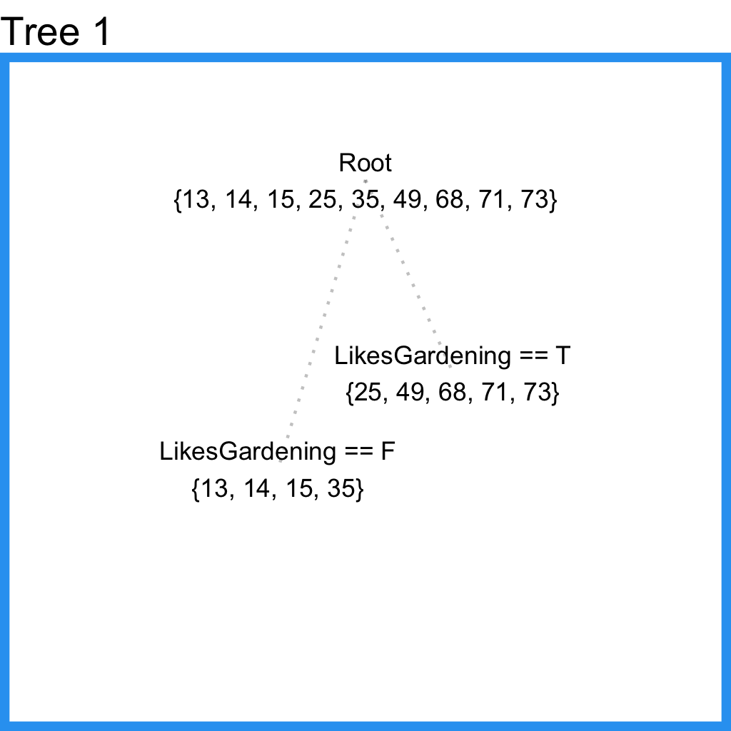
This is nice, but it’s missing valuable information from the feature LikesVideoGames. Let’s try letting terminal nodes have 2 samples.

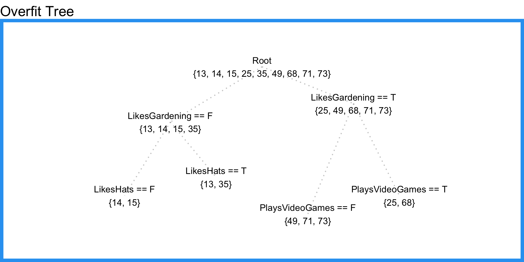
Here we pick up some information from PlaysVideoGames but we also pick up information from LikesHats – a good indication that we’re overfitting and our tree is splitting random noise.

Here in lies the drawback to using a single decision/regression tree – it fails to include predictive power from multiple, overlapping regions of the feature space. Suppose we measure the training errors from our first tree.

PersonID	Age	Tree1 Prediction	Tree1 Residual
1	13	19.25	-6.25
2	14	19.25	-5.25
3	15	19.25	-4.25
4	25	57.20	-32.20
5	35	19.25	15.75
6	49	57.20	-8.20
7	68	57.20	10.80
8	71	57.20	13.80
9	73	57.20	15.80

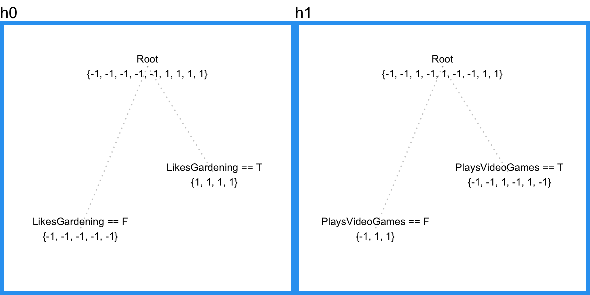
Now we can fit a second regression tree to the residuals of the first tree.

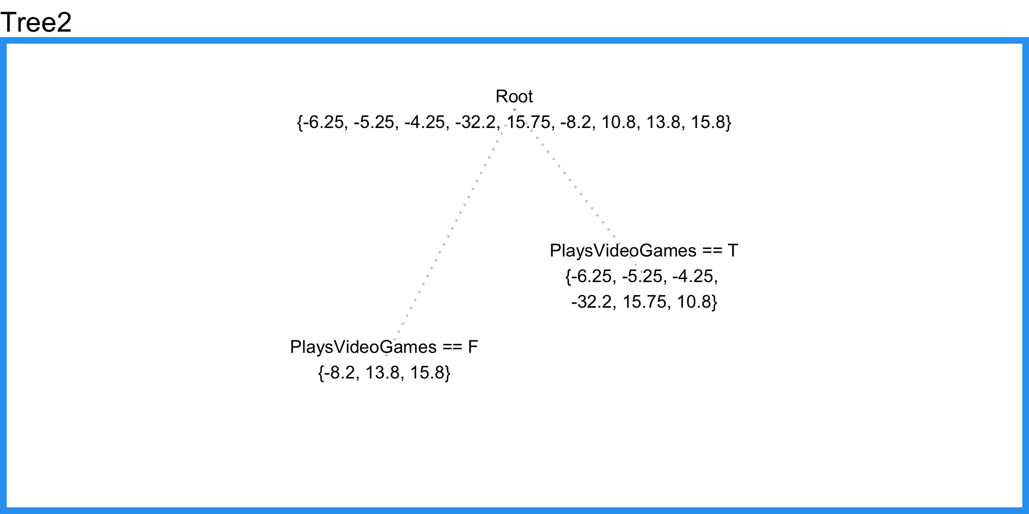
Notice that this tree does not include LikesHats even though our overfitted regression tree above did. The reason is because this regression tree is able to consider LikesHats and PlaysVideoGames with respect to all the training samples, contrary to our overfit regression tree which only considered each feature inside a small region of the input space, thus allowing random noise to select LikesHats as a splitting feature.

Now we can improve the predictions from our first tree by adding the “error-correcting” predictions from this tree.

PersonID	Age	Tree1 Prediction	Tree1 Residual	Tree2 Prediction	Combined Prediction	Final Residual
1	13	19.25	-6.25	-3.57	15.68	2.68
2	14	19.25	-5.25	-3.57	15.68	1.68
3	15	19.25	-4.25	-3.57	15.68	0.68
4	25	57.20	-32.20	-3.57	53.63	28.63
5	35	19.25	15.75	-3.57	15.68	-19.32
6	49	57.20	-8.20	7.13	64.33	15.33
7	68	57.20	10.80	-3.57	53.63	-14.37
8	71	57.20	13.80	7.13	64.33	-6.67
9	73	57.20	15.80	7.13	64.33	-8.67

MSE.Tree1	MSE.Combined
1993.55	1764.57

Draft 1

Inspired by the idea above, we create our first (naive) formalization of gradient boosting. In pseudocode

• Fit a model to the data, $ F_1(x) = y $
• Fit a model to the residuals, $ h_1(x) = y - F_1(x) $
• Create a new model, $ F_2(x) = F_1(x) + h_1(x) $

It’s not hard to see how we can generalize this idea by inserting more models that correct the errors of the previous model. Specifically,

$ F(x) = F_1(x) \mapsto F_2(x) = F_1(x) + h_1(x) \dots \mapsto F_M(x) = F_{M-1}(x) + h_{M-1}(x) $
where $ F_1(x) $ is an initial model fit to $ y $

Since we initialize the procedure by fitting $ F_1(x) $, our task at each step is to find $ h_m(x) = y - F_m(x) $.

Stop. Notice something. $ h_m $ is just a “model”. Nothing in our definition requires it to be a tree-based model. This is one of the broader concepts and advantages to gradient boosting. It’s really just a framework for iteratively improving any weak learner. So in theory, a well coded gradient boosting module would allow you to “plug in” various classes of weak learners at your disposal. In practice however, $ h_m $ is almost always a tree based learner, so for now it’s fine to interpret $ h_m $ as a regression tree like the one in our example.

Draft 2

Now we’ll tweak our model to conform to most gradient boosting implementations - we’ll initialize the model with a single prediction value. Since our task (for now) is to minimize squared error, we’ll initialize $ F $ with the mean of the training target values.

$ F_0(x) = \underset{\gamma}{\arg\min} \sum_{i=1}^n L(y_i, \gamma) = \underset{\gamma}{\arg\min} \sum_{i=1}^n (\gamma - y_i)^2 = {\displaystyle {\frac {1}{n}}\sum {i=1}^{n}y{i}.} $

Then we can define each subsequent $ F_m $ recursively, just like before

$ F_{m+1}(x) = F_m(x) + h_m(x) = y $, for $ m \geq 0 $

where $ h_m $ comes from a class of base learners $ \mathcal{H} $ (e.g. regression trees).

At this point you might be wondering how to select the best value for the model’s hyper-parameter $ m $. In other words, how many times should we iterate the residual-correction procedure until we decide upon a final model, $ F $? This is best answered by testing different values of $ m $ via cross-validation.

Draft 3

Up until now we’ve been building a model that minimizes squared error, but what if we wanted to minimize absolute error? We could alter our base model (regression tree) to minimize absolute error, but this has a couple drawbacks..

• Depending on the size of the data this could be very computationally expensive. (Each considered split would need to search for a median.)
• It ruins our “plug-in” system. We’d only be able to plug in weak learns that support the objective function(s) we want to use.

Instead we’re going to do something much niftier. Recall our example problem. To determine $ F_0 $, we start by choosing a minimizer for absolute error. This’ll be $ median(y) = 35 $. Now we can measure the residuals, $ y - F_0 $.

PersonID	Age	F0	Residual0
1	13	35	-22
2	14	35	-21
3	15	35	-20
4	25	35	-10
5	35	35	0
6	49	35	14
7	68	35	33
8	71	35	36
9	73	35	38

Consider the first and fourth training samples. They have $ F_0 $ residuals of -22 and -10 respectively. Now suppose we’re able to make each prediction 1 unit closer to its target. Respective squared error reductions would be 43 and 19, while respective absolute error reductions would be 1 and 1. So a regression tree, which by default minimizes squared error, will focus heavily on reducing the residual of the first training sample. But if we want to minimize absolute error, moving each prediction one unit closer to the target produces an equal reduction in the cost function. With this in mind, suppose that instead of training $ h_0 $ on the residuals of $ F_0 $, we instead train $ h_0 $ on the gradient of the loss function, $ L(y, F_0(x)) $ with respect to the prediction values produced by $ F_0(x) $. Essentially, we’ll train $ h_0 $ on the cost reduction for each sample if the predicted value were to become one unit closer to the observed value. In the case of absolute error, $ h_m $ will simply consider the sign of every $ F_m $ residual (as apposed to squared error which would consider the magnitude of every residual). After samples in $ h_m $ are grouped into leaves, an average gradient can be calculated and then scaled by some factor, $ \gamma $, so that $ F_m + \gamma h_m $ minimizes the loss function for the samples in each leaf. (Note that in practice, a different factor is chosen for each leaf.)

Gradient Descent

Let’s formalize this idea using the concept of gradient descent. Consider a differentiable function we want to minimize. For example,

$ L(x_1, x_2) = \frac{1}{2}(x_1 - 15)^2 + \frac{1}{2}(x_2 - 25)^2 $

The goal here is to find the pair $ (x_1, x_2) $ that minimizes $ L $. Notice, you can interpret this function as calculating the squared error for two data points, 15 and 25 given two prediction values, $ x_1 $ and $ x_2 $ (but with a $ \frac{1}{2} $ multiplier to make the math work out nicely). Although we can minimize this function directly, gradient descent will let us minimize more complicated loss functions that we can’t minimize directly.

Initialization Steps:

• Number of iteration steps $ M = 100 $
• Starting point $ s^{0} = (0, 0) $
• Step size $ \gamma = 0.1 $

Descent Steps:

For iteration $ m=1 $ to $ M $:

1. Calculate the gradient of $ L $ at the point $ s^{(m-1)} $
2. “Step” in the direction of greatest descent (the negative gradient) with step size $ \gamma $. That is, $ s^{m} = s^{(m-1)} - \gamma \nabla L(s^{(m-1)}) $

If $ \gamma $ is small and $ M $ is sufficiently large, $ s^{M} $ will be the location of $ L $’s minimum value.

A few ways to improve this framework

• Instead of iterating a fixed number of times, we can iterate until the next iteration produces sufficiently small improvement.
• Instead of stepping a fixed magnitude for each step, we can use something like line search smartly choose step sizes.

If you’re struggling with this part, just google gradient descent. It’s been explained many times in many ways.

Leveraging Gradient Descent

Now we can use gradient descent for our gradient boosting model. The objective function we want to minimize is $ L $. Our starting point is $ F_0(x) $. For iteration $ m = 1 $, we compute the gradient of $ L $ with respect to $ F_0(x) $. Then we fit a weak learner to the gradient components. In the case of a regression tree, leaf nodes produce an average gradient among samples with similar features. For each leaf, we step in the direction of the average gradient (using line search to determine the step magnitude). The result is $ F_1 $. Then we can repeat the process until we have $ F_M $.

Take a second to stand in awe of what we just did. We modified our gradient boosting algorithm so that it works with any differentiable loss function. (This is the part that gets butchered by a lot of gradient boosting explanations.) Let’s clean up the ideas above and reformulate our gradient boosting model once again.

Initialize the model with a constant value:
$ F_0(x) = \underset{\gamma}{\arg\min} \sum_{i=1}^n L(y_i, \gamma) $

For m = 1 to M:

1. Compute pseudo residuals, $ r_{im} = -\left[\frac{\partial L(y_i, F(x_i))}{\partial F(x_i)}\right]{F(x)=F{m-1}(x)} \quad \text{for } i=1, \ldots, n $
2. Fit base learner, $ h_{m}(x) $ to pseudo residuals
3. Compute step magnitude multiplier $ \gamma_m $. (In the case of tree models, compute a different $ \gamma_m $ for every leaf.)
4. Update $ F_m(x) = F_{m-1}(x) + \gamma_m h_m(x) $

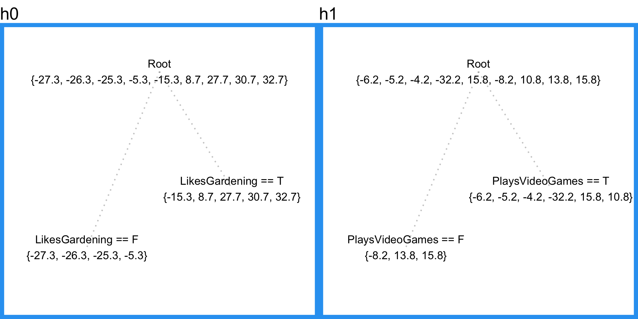
In case you want to check your understanding so far, our current gradient boosting applied to our sample problem for both squared error and absolute error objectives yields the following results.

Squared Error

Age	F0	PseudoResidual0	h0	gamma0	F1	PseudoResidual1	h1	gamma1	F2
13	40.33	-27.33	-21.08	1	19.25	-6.25	-3.57	1	15.68
14	40.33	-26.33	-21.08	1	19.25	-5.25	-3.57	1	15.68
15	40.33	-25.33	-21.08	1	19.25	-4.25	-3.57	1	15.68
25	40.33	-15.33	16.87	1	57.20	-32.20	-3.57	1	53.63
35	40.33	-5.33	-21.08	1	19.25	15.75	-3.57	1	15.68
49	40.33	8.67	16.87	1	57.20	-8.20	7.13	1	64.33
68	40.33	27.67	16.87	1	57.20	10.80	-3.57	1	53.63
71	40.33	30.67	16.87	1	57.20	13.80	7.13	1	64.33
73	40.33	32.67	16.87	1	57.20	15.80	7.13	1	64.33

Absolute Error

Age	F0	PseudoResidual0	h0	gamma0	F1	PseudoResidual1	h1	gamma1	F2
13	35	-1	-1.0	20.5	14.5	-1	-0.33	0.75	14.25
14	35	-1	-1.0	20.5	14.5	-1	-0.33	0.75	14.25
15	35	-1	-1.0	20.5	14.5	1	-0.33	0.75	14.25
25	35	-1	0.6	55.0	68.0	-1	-0.33	0.75	67.75
35	35	-1	-1.0	20.5	14.5	1	-0.33	0.75	14.25
49	35	1	0.6	55.0	68.0	-1	0.33	9.00	71.00
68	35	1	0.6	55.0	68.0	-1	-0.33	0.75	67.75
71	35	1	0.6	55.0	68.0	1	0.33	9.00	71.00
73	35	1	0.6	55.0	68.0	1	0.33	9.00	71.00

Draft 4

<img src="/blog/gradient-boosting-explained_files/george-costanza.jpg" title=“airbnb competition” style=“float:right; width:200px; margin-left:25px; margin-bottom:10px” /> Here we introduce something called shrinkage.

The concept is fairly simple. For each gradient step, the step magnitude is multiplied by a factor between 0 and 1 called a learning rate. In other words, each gradient step is shrunken by some factor. The current Wikipedia excerpt on shrinkage doesn’t mention why shrinkage is effective - it just says that shrinkage appears to be empirically effective. My personal take is that it causes sample-predictions to slowly converge toward observed values. As this slow convergence occurs, samples that get closer to their target end up being grouped together into larger and larger leaves (due to fixed tree size parameters), resulting in a natural regularization effect.

Draft 5

Last up - row sampling and column sampling. Most gradient boosting algorithms provide the ability to sample the data rows and columns before each boosting iteration. This technique is usually effective because it results in more different tree splits, which means more overall information for the model. To get a better intuition for why this is true, check out my post on Random Forest, which employs the same random sampling technique. Alas we have our final gradient boosting framework.

Gradient Boosting in Practice

Gradient boosting in incredibly effective in practice. Perhaps the most popular implementation, XGBoost, is used in a number of winning Kaggle solutions. XGBoost employs a number of tricks that make it faster and more accurate than traditional gradient boosting (particularly 2nd-order gradient descent) so I’ll encourage you to try it out and read Tianqi Chen’s paper about the algorithm. With that said, a new competitor, LightGBM from Microsoft, is gaining significant traction.

What else can it do? Although I presented gradient boosting as a regression model, it’s also very effective as a classification and ranking model. As long as you have a differentiable loss function for the algorithm to minimize, you’re good to go. Common objective functions include cross entropy for classification and mean squared error for regression.

I leave you with a quote from my fellow Kaggler Mike Kim.

My only goal is to gradient boost over myself of yesterday. And to repeat this everyday with an unconquerable spirit.