Introduction To Neural Networks

Artificial Neural Networks are all the rage. One has to wonder if the catchy name played a role in the model’s own marketing and adoption. I’ve seen business managers giddy to mention that their products use “Artificial Neural Networks” and “Deep Learning”. Would they be so giddy to say their products use “Connected Circles Models” or “Fail and Be Penalized Machines”? But make no mistake – Artificial Neural Networks are the real deal as evident by their success in a number of applications like image recognition, natural language processing, automated trading, and autonomous cars. As a professional data scientist who didn’t fully understand them, I felt embarrassed like a builder without a table saw. Consequently I’ve done my homework and written this article to help others overcome the same hurdles and head scratchers I did in my own (ongoing) learning process.

Note that R code for the examples presented in this article can be found here in the Machine Learning Problem Bible. Additionally, check out Part 2, Neural Networks – A Worked Example after reading this article to see the details behind designing and coding a neural network from scratch.

We’ll start with a motivational problem. Here we have a collection of grayscale images, each a 2×2 grid of pixels where each pixel has an intensity value between 0 (white) and 255 (black). The goal is to build a model that identifies images with a “stairs” pattern.

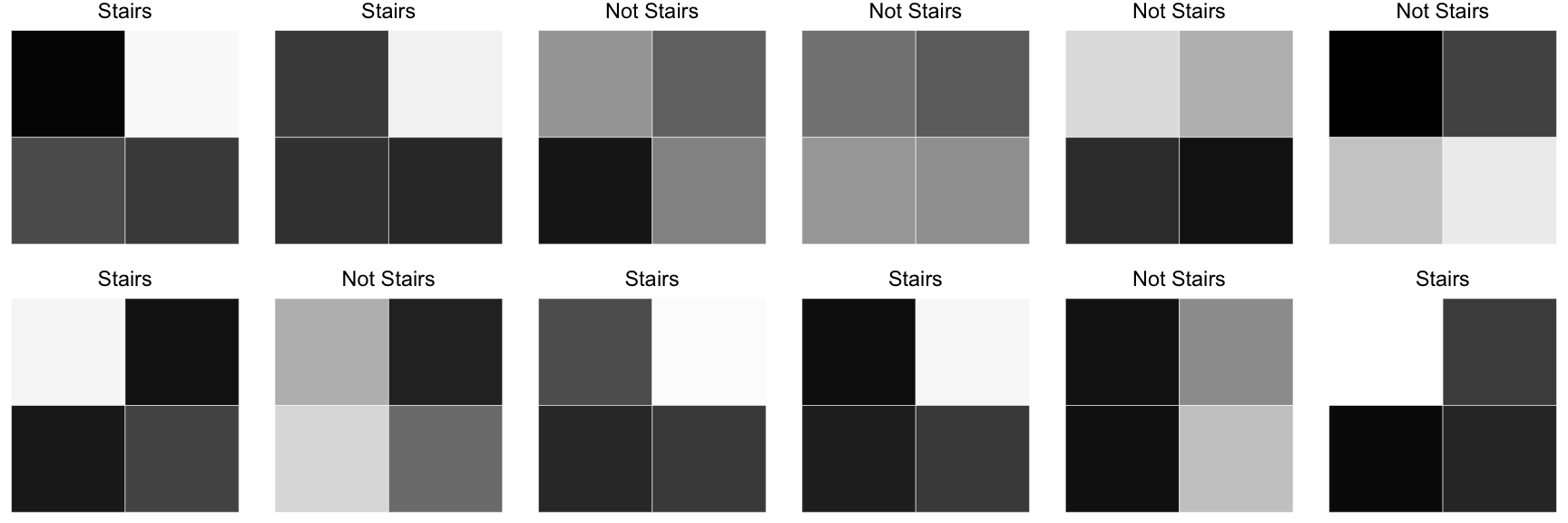
At this point, we are only interested in finding a model that could fit the data reasonably. We’ll worry about the fitting methodology later.

Pre-processing

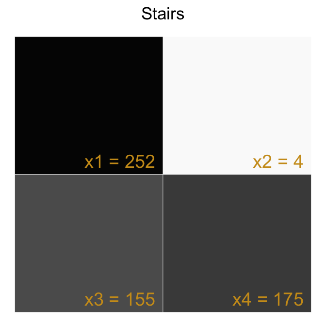
For each image, we label the pixels $ x_1 $, $ x_2 $, $ x_3 $, $ x_4 $ and generate an input vector $ \mathbf{x} = \begin{bmatrix}x_1 & x_2 & x_3 & x_4\end{bmatrix} $ which will be the input to our model. We expect our model to predict True (the image has the stairs pattern) or False (the image does not have the stairs pattern).

ImageId	x1	x2	x3	x4	IsStairs
1	252	4	155	175	1
2	175	10	186	200	1
3	82	131	230	100	0
...	...	...	...	...	...
498	36	187	43	249	0
499	1	160	169	242	1
500	198	134	22	188	0

Single Layer Perceptron (Model Iteration 0)

A simple model we could build is a single layer perceptron. A perceptron uses a weighted linear combination of the inputs to return a prediction score. If the prediction score exceeds a selected threshold, the perceptron predicts True. Otherwise it predicts False. More formally,

$$ f(x)={\begin{cases} 1 &{\text{if }}\ w_1x_1 + w_2x_2 + w_3x_3 + w_4x_4 > threshold \\ 0 & {\text{otherwise}} \end{cases}} $$

Let’s re-express this as follows

$$ \widehat y = \mathbf w \cdot \mathbf x + b $$

$$ f(x)={\begin{cases} 1 &{\text{if }}\ \widehat{y} > 0 \\ 0 & {\text{otherwise}} \end{cases}} $$

Here $ \widehat{y} $ is our prediction score.

Pictorially, we can represent a perceptron as input nodes that feed into an output node.

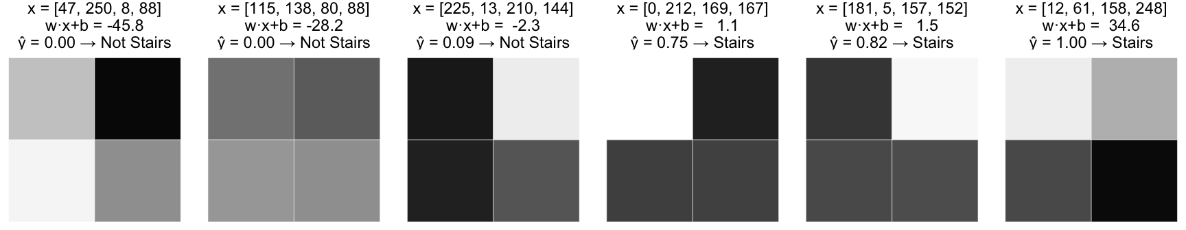
For our example, suppose we build the following perceptron:

$$ \widehat{y} = -0.0019x_1 + -0.0016x_2 + 0.0020x_3 + 0.0023x_4 + 0.0003 $$

Here’s how the perceptron would perform on some of our training images.

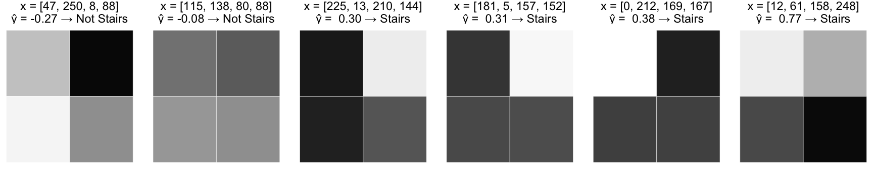
This would certainly be better than randomly guessing and it makes some logical sense. All the stairs patterns have darkly shaded pixels in the bottom row which supports the larger, positive coefficients for $ x_3 $ and $ x_4 $. Nonetheless, there are some glaring problems with this model.

• The model outputs a real number whose value correlates with the concept of likelihood (higher values imply a greater probability the image represents stairs) but there’s no basis to interpret the values as probabilities, especially since they can be outside the range [0, 1].
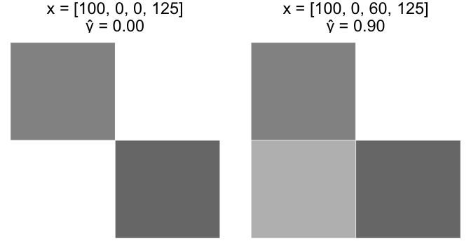
• The model can’t capture the non-linear relationship between the variables and the target. To see this, consider the following hypothetical scenarios

Case A

Start with an image, x = [100, 0, 0, 125]. Increase $ x_3 $ from 0 to 60.

Case B

Start with the last image, x = [100, 0, 60, 125]. Increase $ x_3 $ from 60 to 120.

Intuitively, Case A should have a much larger increase in $ \widehat y $ than Case B. However, since our perceptron model is a linear equation, the equivalent +60 change in $ x_3 $ resulted in an equivalent +0.12 change in $ \widehat y $ for both cases.

There are more issues with our linear perception, but let’s start by addressing these two.

Single Layer Perceptron with Sigmoid activation function (Model Iteration 1)

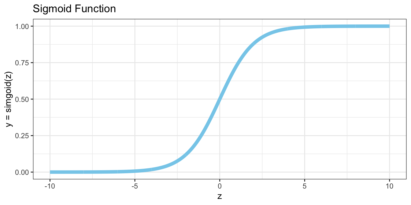
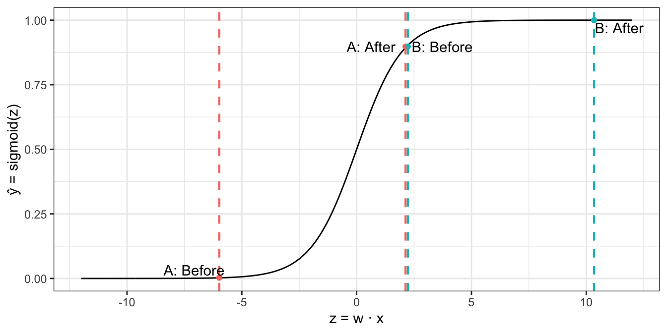
We can fix problems 1 and 2 above by wrapping our perceptron within a sigmoid function (and subsequently choosing different weights). Recall that the sigmoid function is an S shaped curve bounded on the vertical axis between 0 and 1, and is thus frequently used to model the probability of a binary event.

$$ sigmoid(z) = \frac{1}{1 + e^{-z}} $$

Following this idea, we can update our model with the following picture and equation.

$$ z = w \cdot x = w_1x_1 + w_2x_2 + w_3x_3 + w_4x_4 $$

$$ \widehat y = sigmoid(z) = \frac{1}{1 + e^{-z}} $$

Looks familiar? It’s our old friend, logistic regression. However, it’ll serve us well to interpret the model as a linear perceptron with a sigmoid “activation function” because that gives us more room to generalize. Also, since we now interpret $ \widehat y $ as a probability, we must update our decision rule accordingly.

$$ f(x)={\begin{cases} 1 &{\text{if }}\ \widehat{y} > 0.5 \\ 0 & {\text{otherwise}} \end{cases}} $$

Continuing with our example problem, suppose we come up with the following fitted model:

$$ \begin{bmatrix} w_1 & w_2 & w_3 & w_4 \end{bmatrix} = \begin{bmatrix} -0.140 & -0.145 & 0.121 & 0.092 \end{bmatrix} $$

$$ b = -0.008 $$

$$ \widehat y = \frac{1}{1 + e^{-(-0.140x_1 -0.145x_2 + 0.121x_3 + 0.092x_4 -0.008)}} $$

Observe how this model performs on the same sample images from the previous section.

Clearly this fixes problem 1 from above. Observe how it also fixes problem 2.

Case A

Start with an image, x = [100, 0, 0, 125]. Increase $ x_3 $ from 0 to 60.

Case B

Start with the last image, x = [100, 0, 60, 125]. Increase $ x_3 $ from 60 to 120.

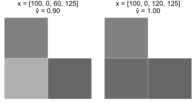
Notice how the curvature of the sigmoid function causes Case A to “fire” (increase rapidly) as $ z = w \cdot x $ increases, but the pace slows down as $ z $ continues to increase. This aligns with our intuition that Case A should reflect a greater increase in the likelihood of stairs versus Case B.

Unfortunately this model still has issues.

1. $ \widehat y $ has a monotonic relationship with each variable. What if we want to identify lightly shaded stairs?
2. The model does not account for variable interaction. Assume the bottom row of an image is black. If the top left pixel is white, darkening the top right pixel should increase the probability of stairs. If the top left pixel is black, darkening the top right pixel should decrease the probability of stairs. In other words, increasing $ x_3 $ should potentially increase or decrease $ \widehat y $ depending on the values of the other variables. Our current model has no way of achieving this.

Multi-Layer Perceptron with Sigmoid activation function (Model Iteration 2)

We can solve both of the above issues by adding an extra layer to our perceptron model. We’ll construct a number of base models like the one above, but then we’ll feed the output of each base model as input into another perceptron. This model is in fact a vanilla neural network. Let’s see how it might work on some examples.

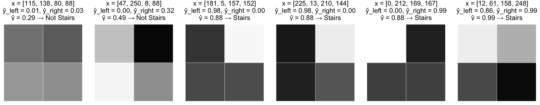
Example 1: Identify the stairs pattern

• Build a model that fires when “left stairs” are identified, $ \widehat y_{left} $
• Build a model that fires when “right stairs” are identified, $ \widehat y_{right} $
• Add the score of the base models so that the final sigmoid function only fires if both $ \widehat y_{left} $ and $ \widehat y_{right} $ are large

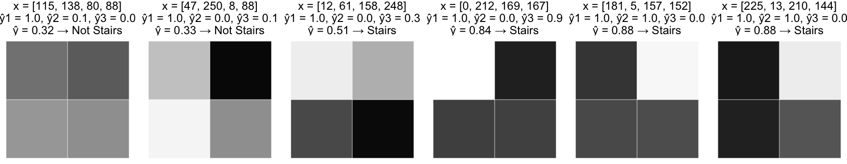
Alternatively

1. Build a model that fires when the bottom row is dark, $ \widehat y_1 $
2. Build a model that fires when the top left pixel is dark and the top right pixel is light, $ \widehat y_2 $
3. Build a model that fires when the top left pixel is light and the top right pixel is dark, $ \widehat y_3 $
4. Add the base models so that the final sigmoid function only fires if $ \widehat y_1 $ and $ \widehat y_2 $ are large, or $ \widehat y_1 $ and $ \widehat y_3 $ are large. (Note that $ \widehat y_2 $ and $ \widehat y_3 $ cannot both be large)

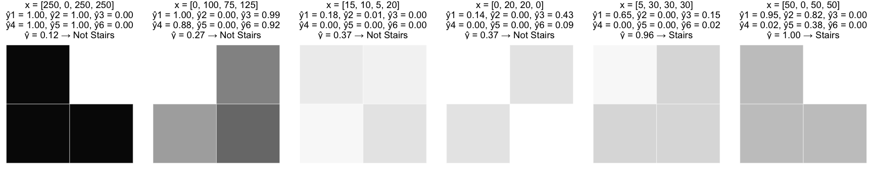
Example 2: Identify lightly shaded stairs

1. Build models that fire for “shaded bottom row”, “shaded x1 and white x2”, “shaded x2 and white x1”, $ \widehat y_1 $, $ \widehat y_2 $, and $ \widehat y_3 $
2. Build models that fire for “dark bottom row”, “dark x1 and white x2”, “dark x2 and white x1”, $ \widehat y_4 $, $ \widehat y_5 $, and $ \widehat y_6 $
3. Combine the models so that the “dark” identifiers are essentially subtracted from the “shaded” identifiers before squashing the result with a sigmoid function

A note about terminology

A single-layer perceptron has a single output layer. Consequently, the models we just built would be called two-layer perceptrons because they have an output layer which is the input to another output layer. However, we could call these same models neural networks, and in this respect the networks have three layers - an input layer, a hidden layer, and an output layer.

Alternative activation functions

In our examples we used a sigmoid activation function. However, we could use other activation functions. tanh and relu are common choices. The activation function must be non-linear, otherwise the neural network would simplify to an equivalent single layer perceptron.

Multiclass classification

We can easily extend our model to work for multiclass classification by using multiple nodes in the final output layer. The idea here is that each output node corresponds to one of the $ C $ classes we are trying to predict. Instead of squashing the output with the sigmoid function which maps an element in $ \mathbb{R} $ to and element in [0, 1], we can use the softmax function which maps a vector in $ \mathbb{R}^n $ to a vector in $ \mathbb{R}^n $ such that the resulting vector elements sum to 1. In other words, we can design the network such that it outputs the vector [$ prob(class_1) $, $ prob(class_2) $, …, $ prob(class_C) $].

Using more than two layers (Deep Learning)

You might be wondering, “Can we extend our vanilla neural network so that its output layer is fed into a 4th layer (and then a 5th, and 6th, etc.)?”. Yes. This is what’s commonly referred to as “deep learning”. In practice it can be very effective. However, it’s worth noting that any network you build with more than one hidden layer can be mimicked by a network with only one hidden layer. In fact, you can approximate any continuous function using a neural network with a single hidden layer as per the Universal Approximation Theorem. The reason deep neural network architectures are frequently chosen in favor of single hidden layer architectures is that they tend to converge to a solution faster during the fitting procedure.

Fitting the model to labeled training samples (Backpropagation)

Alas we come to the fitting procedure. So far we’ve discussed how neural networks could work effectively, but we haven’t discussed how to fit a neural network to labeled training samples. An equivalent question would be, “How can we choose the best weights for a network, given some labeled training samples?”. Gradient descent is the common answer (although MLE can work too). Continuing with our example problem, the gradient descent procedure would go something like this:

1. Start with some labeled training data
2. Choose a differentiable loss function to minimize, $ L(\mathbf{\widehat Y}, \mathbf{Y}) $
3. Choose a network structure. Specifically detemine how many layers and how many nodes in each layer.
4. Initialize the network’s weights randomly
5. Run the training data through the network to generate a prediction for each sample. Measure the overall error according to the loss function, $ L(\mathbf{\widehat Y}, \mathbf{Y}) $. (This is called forward propagation)
6. Determine how much the current loss will change with respect to a small change in each of the weights. In other words, calculate the gradient of $ L $ with respect to every weight in the network. (This is called backward propagation)
7. Take a small “step” in the direction of the negative gradient. For example, if $ w_{23} = 1.5 $ and $ \frac{\partial L}{\partial w_{23}} = 2.2 $, then decreasing $ w_{23} $ by a small amount should result in a small decrease in the current loss. Hence we update $ w_{23} := w_{23} - 2.2 \times 0.001 $ (where 0.001 is our predetermined “step size”).
8. Repeat this process (from step 5) a fixed number of times or until the loss converges

That’s the basic idea at least. In practice, this poses a number of challenges.

Challenge 1 - Computational Complexity

During the fitting procedure, one of the things we’ll need to calculate is the gradient of $ L $ with respect to every weight. This is tricky because $ L $ depends on every node in the output layer, and each of those nodes depends on every node in the layer before it, and so on. This means calculating $ \frac{\partial L}{\partial w_{ab}} $ is a chain-rule nightmare. (Keep in mind that many real-wold neural networks have thousands of nodes across tens of layers.) The key to dealing with this is to recognize that most of the $ \frac{\partial L}{\partial w_{ab}} $s reuse the same intermediate derivatives when you apply the chain-rule. If you’re careful about tracking this, you can avoid recalculating the same thing thousands of times.

Another trick is to use special activation functions whose derivatives can be written as a function of their value. For example, the derivative of $ sigmoid(x) $ = $ sigmoid(x)(1 - sigmoid(x)) $. This is convenient because during the forward pass, when we calculate $ \widehat y $ for each training sample, we have to calculate $ sigmoid(\mathbf{x}) $ element-wise for some vector $ \mathbf{x} $. During backprop we can reuse those values when calculating the gradient of $ L $ with respect to the weights, saving time and memory.

A third trick is to partition the training data into “mini batches” and update the weights with respect to each batch, one after another. For example, if you partition your training data into {batch1, batch2, batch3}, the first pass over the training data would

1. Update the weights using batch1
2. Update the weights using batch2
3. Update the weights using batch3

where the gradient of $ L $ is recalculated after each update.

The last technique worth mentioning is to make use of GPU as opposed to CPU, as GPU is better suited to perform lots of calculations in parallel.

Challenge 2 - Gradient Descent may have trouble finding the absolute minimum

This is not so much a neural network problem as it is a gradient descent problem. It’s possible that the weights could get stuck in a local minimum during gradient descent. It’s also possible that weights can overshoot the minimum. One trick to dealing with this is to tinker with different step sizes. Another trick is to increase the number of nodes and/or layers in the network. (Beware of overfitting). Additionally, some heuristic techniques like using momentum can be effective.

Challenge 3 - How to generalize?

How might we write a generic program to fit any neural network with any number of nodes and layers? The answer is, “You don’t. You use Tensorflow”. But if you really wanted to, the hard part is calculating the gradient of the loss function. The trick to doing this is to recognize that you can represent the gradient as a recursive function. A neural network with 5 layers is just a neural network with 4 layers that feeds into some perceptrons. But a neural network with 4 layers is just a neural network with 3 layers that feed into some perceptrons. And so on it goes. This is more formally known as auto differentiation.

Now check out Neural Networks - A Worked Example to see how to build a neural network from scratch.