Guide to Model Stacking (i.e. Meta Ensembling)

2016-12-13 2301 words 11 minutes

Contents

Introduction

Stacking (also called meta ensembling) is a model ensembling technique used to combine information from multiple predictive models to generate a new model. Often times the stacked model (also called 2nd-level model) will outperform each of the individual models due its smoothing nature and ability to highlight each base model where it performs best and discredit each base model where it performs poorly. For this reason, stacking is most effective when the base models are significantly different. Here I provide a simple example and guide on how stacking is most often implemented in practice.

Feel free to follow this article using the related code and datasets in the Machine Learning Problem Bible.

Motivation

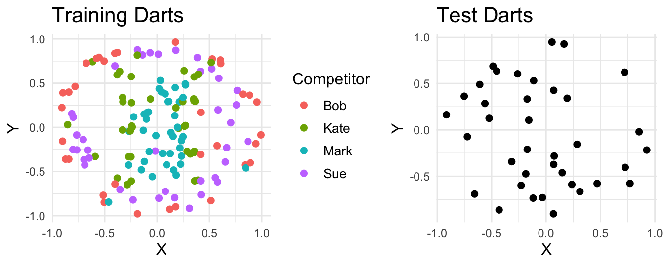
Suppose four people throw a combined 187 darts at a board. For 150 of those we get to see who threw each dart and where it landed. For the rest, we only get to see where the dart landed. Our task is to guess who threw each of the unlabelled darts based on their landing spot.

K-Nearest Neighbors (Base Model1)

Let’s make a sad attempt at solving this classification problem using a K-Nearest Neighbors model. In order to select the best value for K, we’ll use 5-fold Cross-Validation combined with Grid Search where K = (1, 2, … 30). In pseudo code,

Partition the training data into five equal size folds. Call these test folds
For K = 1, 2, … 30
1. For each test fold
  1. Combine the other four folds to be used as a training fold
  2. Fit a K-Nearest Neighbors model on the training fold (using the current value of K)
  3. Make predictions on the test fold and measure the resulting accuracy rate of the predictions
2. Calculate the average accuracy rate from the five test fold predictions
Keep the K value with the best average CV accuracy rate

With our fictitious data we find K = 1 to have the best CV performance (67% accuracy). Using K = 1, we now train a model on the entire training dataset and make predictions on the test dataset. Ultimately this will give us about 70% classification accuracy.

Support Vector Machine (Base Model2)

Now let’s make another sad attempt at solving the problem using a Support Vector Machine. Additionally, we’ll add a feature DistFromCenter that measures the distance each point lies from the center of the board to help make the data linearly separable. With R’s LiblineaR package we get two hyper parameters to tune:

type

L2-regularized L2-loss support vector classification (dual)
L2-regularized L2-loss support vector classification (primal)
L2-regularized L1-loss support vector classification (dual)
support vector classification by Crammer and Singer
L1-regularized L2-loss support vector classification

cost

Inverse of the regularization constant

The grid of parameter combinations we’ll test is the cartesian product of the 5 listed SVM types with cost values of (.01, .1, 1, 10, 100, 1000, 2000). That is

type	cost
1	0.01
1	0.1
1	1
...	...
5	100
5	1000
5	2000

Using the same CV + Grid Search approach we used for our K-Nearest Neighbors model, here we find the best hyper-parameters to be type = 4 with cost = 1000. Again, we use these parameters to train a model on the full training dataset and make predictions on the test dataset. This’ll give us about 61% CV classification accuracy and 78% classification accuracy on the test dataset.

Stacking (Meta Ensembling)

Let’s take a look at the regions of the board each model would classify as Bob, Sue, Mark, or Kate.

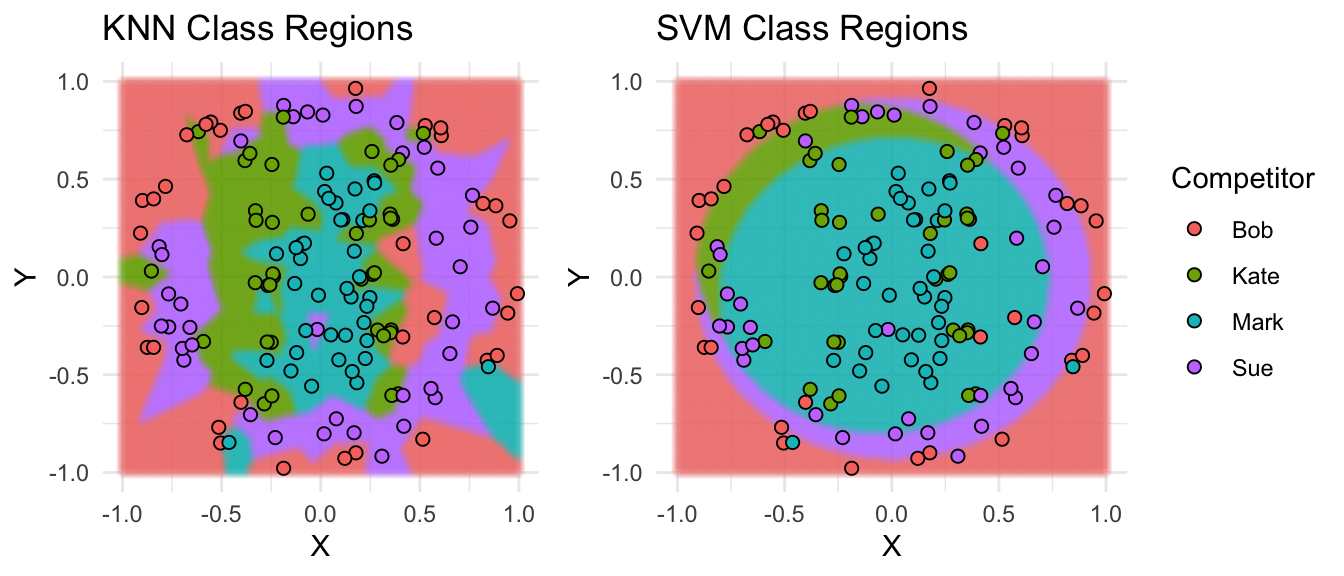
Unsurprisingly, the KNN model does a good job at classifying Kate’s throws and Mark’s throws but does poorly at separating Bobs’s throws and Sue’s throws. The opposite appears to be true for the SVM model. HINT: Stacking these models will probably be fruitful.

There are a few schools of thought on how to actually implement stacking. Here’s my personal favorite applied to our example problem.

1. Partition the training dataset

into five test folds

ID	FoldID	X	Y	DistFromCenter	Competitor
1	5	-0.4	-0.64	0.76	Bob
3	5	0.32	-0.3	0.44	Kate
4	4	0.53	0.77	0.94	Bob
...	...	...	...	...	...
185	2	0.13	-0.06	0.14	Mark
186	2	0.52	0.73	0.9	Kate
187	3	0.7	0.05	0.71	Sue

2. Create a dataset called train_meta

with the same row Ids and fold Ids as the training dataset, with empty columns M1 and M2. Similarly create a dataset called test_meta with the same row Ids as the test dataset and empty columns M1 and M2

train_meta
ID	FoldID	X	Y	DistFromCenter	M1	M2	Competitor
1	5	-0.4	-0.64	0.76			Bob
3	5	0.32	-0.3	0.44			Kate
4	4	0.53	0.77	0.94			Bob
...	...	...	...	...	...	...	...
185	2	0.13	-0.06	0.14			Mark
186	2	0.52	0.73	0.9			Kate
187	3	0.7	0.05	0.71			Sue

test_meta
ID	X	Y	DistFromCenter	M1	M2	Competitor
2	-0.03	-0.73	0.73			Sue
5	-0.61	0.49	0.78			Sue
9	0.73	-0.4	0.83			Sue
...	...	...	...	...	...	...
173	-0.11	0.53	0.54			Mark
174	0.07	0.43	0.43			Mark
175	-0.32	-0.34	0.47			Kate

3. For each test fold…

Fold1, Fold2, … Fold5

3.1 Combine the other four folds

to be used as a training fold

train-fold 1
ID	FoldID	X	Y	DistFromCenter	Competitor
1	5	-0.4	-0.64	0.76	Bob
3	5	0.32	-0.3	0.44	Kate
4	4	0.53	0.77	0.94	Bob
...	...	...	...	...	...
185	2	0.13	-0.06	0.14	Mark
186	2	0.52	0.73	0.9	Kate
187	3	0.7	0.05	0.71	Sue

3.2 For each base model

M1: K-Nearest Neighbors (k = 1)
M2: Support Vector Machine (type = 4, cost = 1000)

3.2.1 Fit the base model to the training fold

and make predictions on the test fold. Store these predictions in train_meta to be used as features for the stacking model

train_meta
ID	FoldID	X	Y	DistFromCenter	M1	M2	Competitor
1	5	-0.4	-0.64	0.76			Bob
3	5	0.32	-0.3	0.44			Kate
4	4	0.53	0.77	0.94			Bob
...	...	...	...	...	...	...	...
185	2	0.13	-0.06	0.14			Mark
186	2	0.52	0.73	0.9			Kate
187	3	0.7	0.05	0.71			Sue

4. Fit each base model to the full training dataset

and make predictions on the test dataset. Store these predictions inside test_meta

test_meta
ID	X	Y	DistFromCenter	M1	M2	Competitor
2	-0.03	-0.73	0.73	Sue	Sue	Sue
5	-0.61	0.49	0.78	Bob	Kate	Sue
9	0.73	-0.4	0.83	Sue	Sue	Sue
...	...	...	...	...	...	...
173	-0.11	0.53	0.54	Kate	Mark	Mark
174	0.07	0.43	0.43	Mark	Mark	Mark
175	-0.32	-0.34	0.47	Kate	Mark	Kate

5. Fit a new model, S

(i.e the stacking model) to train_meta, using M1 and M2 as features. Optionally, include other features from the original training dataset or engineered features

6. Use the stacked model S

to make final predictions on test_meta

test_meta
ID	X	Y	DistFromCenter	M1	M2	Pred	Competitor
2	-0.03	-0.73	0.73	Sue	Sue	Sue	Sue
5	-0.61	0.49	0.78	Bob	Kate	Sue	Sue
9	0.73	-0.4	0.83	Sue	Sue	Sue	Sue
...	...	...	...	...	...	...	...
173	-0.11	0.53	0.54	Kate	Mark	Kate	Mark
174	0.07	0.43	0.43	Mark	Mark	Mark	Mark
175	-0.32	-0.34	0.47	Kate	Mark	Kate	Kate

The main point to take home is that we’re using the predictions of the base models as features (i.e. meta features) for the stacked model. So, the stacked model is able to discern where each model performs well and where each model performs poorly. It’s also important to note that the meta features in row i of train_meta are not dependent on the target value in row i because they were produced using information that excluded the target_i in the base models’ fitting procedure.

Alternatively, we could make predictions on the test dataset using each base model immediately after it gets fit to each test fold. In our case this would generate test-set predictions for five K-Nearest Neighbors models and five SVM models. Then we would average the predictions per model to generate our M1 and M2 meta features. One benefit to this is that it’s less time consuming than the first approach (since we don’t have to retrain each model on the full training dataset). It also helps that our train meta features and test meta features should follow a similar distribution. However, the test metas M1 and M2 are likely more accurate in the first approach since each base model was trained on the full training dataset (as opposed to 80% of the training dataset, five times in the 2nd approach).

Stacked Model Hyper Parameter Tuning

So, how do you tune the hyper parameters of the stacked model? Regarding the base models, we can tune their hyper parameters using Cross-Validation + Grid Search just like we did earlier. It doesn’t really matter what folds we use, but it’s usually convenient to use the same folds that we use for stacking. Tuning the hyper parameters of the stacked model is where things get interesting. In practice most people (including myself) simply use Cross Validation + Grid Search using the same exact CV folds used to generate the Meta Features. There’s a subtle flaw to this approach – can you spot it?

Indeed, there’s a small bit of data leakage in our stacking CV procedure. Consider the 1st round of Cross Validation for the stacked model. We fit a model S to {fold2, fold3, fold4, fold5}, make predictions on fold1 and evaluate performance. But the meta features in {fold2, fold3, fold4, fold5} are dependent on the target values in fold1. So, the target values we’re trying to predict are themselves embedded into the features we’re using to fit our model. This is leakage and in theory S could deduce information about the target values from the meta features in a way that would cause it to overfit the training data and not generalize well to out-of-bag samples. However, you have to work hard to conjure up an example where this leakage is significant enough to cause the stacked model to overfit. In practice, everyone ignores this theoretical hole (and frankly I think most people are unaware it even exists!).

Stacking Model Selection and Features

How do you know what model to choose as the stacker and what features to include with the meta features? In my opinion, this is more of an art than a science. Your best bet is to try different things and familiarize yourself with what works and what doesn’t. Another question is, what (if any) other features should you include in for the stacking model in addition to the meta features? Again this is somewhat of an art. Looking at our example, it’s pretty evident that DistFromCenter plays a part in determining which model will perform well. The KNN appears to do better at classifying darts thrown near the center and the SVM model does better at classifying darts thrown away from the center. Let’s take a shot at stacking our models using Logistic Regression. We’ll use the base model predictions as meta features and DistFromCenter as an additional feature.

[Code you can’t see]

Sure enough the stacked model performs better than both of the base models – 75% CV accuracy and 86% test accuracy. Now let’s take a look at its classification regions overlaying the training data, just like we did with the base models.

stacked-model-train-class-regions2

The takeaway here is that the Logistic Regression Stacked Model captures the best aspects of each base model which is why it performs better than either base model in isolation.

Stacking in Practice

To wrap this up, let’s talk about how, when, and why you might use stacking in the real world. Personally, I mostly use stacking in machine learning competitions on Kaggle In general, stacking produces small gains with a lot of added complexity – not worth it for most businesses. But Stacking is almost always fruitful so it’s almost always used in top Kaggle solutions. In fact, stacking is really effective on Kaggle when you have a team of people trying to collaborate on a model. A single set of folds is agreed upon and then every team member builds their own model(s) using those folds. Then each model can be combined using a single stacking script. This is great because it prevents team members from stepping on each others toes, awkwardly trying to stitch their ideas into the same code base.

One last bit. Suppose we have dataset with (user, product) pairs and we want to predict the probability that a user will purchase a given product if he/she is presented an ad with that product. An effective feature might be something like, using the training data, what percent of the products advertised to a user did he actually purchase in the past? So, for the sample (user1, productA) in the training data, we want to tack on a feature like UserPurchasePercentage but we have to be careful not to introduce leakage into the data. We do this as follows

Split the training data into folds
For each test fold
1. Identify the unique set of users in the test fold
2. Use the remaining folds to calculate UserPurchasePercentage (percent of advertised products each user purchased)
3. Map UserPurchasePercentage back to the training data via (fold id, user id)

Now we can use UserPurchasePercentage as a feature for our gradient boosting model (or whatever model we want). Effectively what we’ve just done is built a predictive model that predicts \(user_i\) will purchase \(product_x\) with probability based on the percent of advertised products he purchased in the past and used those predictions as a meta feature for our real model. This is a subtle but valid and effective form of stacking – one which I often do implement in practice and on Kaggle.