Convert More Sales Leads With Machine Learning
The Problem
You sell software that helps stores manage their inventory. You collect leads on thousands of potential customers, and your strategy is to cold-call them and pitch your product. You can only make 100 phone calls per day, so you want to identify leads with a high probability of converting to a sale. By calling leads randomly, you only generate about two sales per day - a 2% hit ratio. If you could be smarter about who you target, you could increase your sales with no extra resources…
The Solution
Machine Learning. You tracked important data on your leads – attributes like Facebook likes, phone number, type of business, etc. Now you can use machine learning techniques to build a model to help you separate the strong leads from the weak ones. In this article I’ll present an example dataset with example solutions to illustrate how this works. If you’d like to download the data and solutions, you can find them in the Rank Sales Leads directory of the Machine Learning Problem Bible on Github.
The Data
train
| LeadID | CompanyName | TypeOfBusiness | FacebookLikes | TwitterFollowers | Website | PhoneNumber | Contact | Sale |
|---|---|---|---|---|---|---|---|---|
| 1 | Drugs R Us | drug store | NA | NA | NA | 5042538336 | general line | FALSE |
| 4 | Joe's Hobby Shop | hobbies & toys | NA | NA | NA | 5043304798 | other | FALSE |
| 5 | The Corner | corner store | 26 | NA | thecornerstore.com | 6461045953 | owner | TRUE |
| ... | ... | ... | ... | ... | ... | ... | ... | ... |
| 26 | Juicy Burger | restaurant | 112 | 20 | NA | 3103833242 | other | FALSE |
| 27 | Comic Corner | books | 89 | 67 | comiccorner.com | 5044820790 | manager | TRUE |
| 28 | Smokes and Beer | corner store | NA | NA | NA | 5046995720 | other | FALSE |
test
| LeadID | CompanyName | TypeOfBusiness | FacebookLikes | TwitterFollowers | Website | PhoneNumber | Contact | Sale |
|---|---|---|---|---|---|---|---|---|
| 2 | The Law Offices of Smith | law office | 87 | 46 | smithlaw.net | 3109859670 | other | FALSE |
| 3 | Bait n Tackle | NA | 22 | NA | NA | 6464315297 | owner | TRUE |
| 6 | Smokie's Bar & Grill | restaurant | 215 | NA | NA | 6461572195 | general line | FALSE |
| ... | ... | ... | ... | ... | ... | ... | ... | ... |
| 22 | Tools & Supplies | NA | NA | NA | NA | 3101508786 | owner | FALSE |
| 29 | Reading Rainbow | books | 6 | NA | readingrainbowstore.us | 5049169286 | owner | FALSE |
| 30 | Katz Claims | law office | 144 | 36 | katzclaims.com | 5045337861 | owner | FALSE |
The Objective
This is important! The simplest and most common objective function for most binary classification algorithms is accuracy rate. This is not what we want. For our sample training dataset, just 35% of leads convert to a sale and in practice this number can be much lower (less than 1%). The most accurate model will often be the one that predicts every lead will not become a sale. Instead, we’re interested in accurately ranking the likelihood that each lead becomes a sale. Then we can pick out the best leads to pursue with confidence that our overall conversion rate will be higher than pursuing a set of random leads. A very easy and common objective function for this is Area Under the ROC Curve. There’s a lot of information about it, so I encourage you to Google it.
In short…
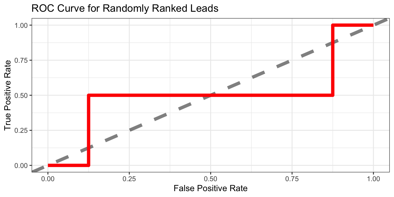
Suppose we randomly sort our leads and predict that every lead converts to a sale. Then we can measure the cumulative True Positive Rate (portion of sales correctly identified up to position i) and the cumulative False Positive Rate (portion of non-sales incorrectly identified up to position i). Now we can plot the cumulative True Positive Rate vs the cumulative False Positive Rate which, in theory, will generate a $ y = x $ line from 0 to 1. So, for a point (x, y) like (0.5, 0.5), the interpretation is that we have to pursue 50% of the total non-converting leads in order to catch 50% of converting leads.
| LeadID | Sale | Prediction | FalsePositiveRate | TruePositiveRate |
|---|---|---|---|---|
| 12 | FALSE | TRUE | 0.125 | 0.0 |
| 13 | TRUE | TRUE | 0.125 | 0.5 |
| 6 | FALSE | TRUE | 0.250 | 0.5 |
| 22 | FALSE | TRUE | 0.375 | 0.5 |
| 19 | FALSE | TRUE | 0.500 | 0.5 |
| 11 | FALSE | TRUE | 0.625 | 0.5 |
| 30 | FALSE | TRUE | 0.750 | 0.5 |
| 29 | FALSE | TRUE | 0.875 | 0.5 |
| 3 | TRUE | TRUE | 0.875 | 1.0 |
| 2 | FALSE | TRUE | 1.000 | 1.0 |
Now suppose we build a model that predicts the probability each lead will convert. We sort the data from the strongest lead to the weakest lead and remeasure the cumulative True Positive Rate and True Negative Rate. Plotting this over our previous example yields
| LeadID | Sale | Prediction | FalsePositiveRate | TruePositiveRate |
|---|---|---|---|---|
| 19 | FALSE | TRUE | 0.125 | 0.0 |
| 3 | TRUE | TRUE | 0.125 | 0.5 |
| 6 | FALSE | TRUE | 0.250 | 0.5 |
| 13 | TRUE | TRUE | 0.250 | 1.0 |
| 30 | FALSE | TRUE | 0.375 | 1.0 |
| 29 | FALSE | TRUE | 0.500 | 1.0 |
| 2 | FALSE | TRUE | 0.625 | 1.0 |
| 11 | FALSE | TRUE | 0.750 | 1.0 |
| 22 | FALSE | TRUE | 0.875 | 1.0 |
| 12 | FALSE | TRUE | 1.000 | 1.0 |
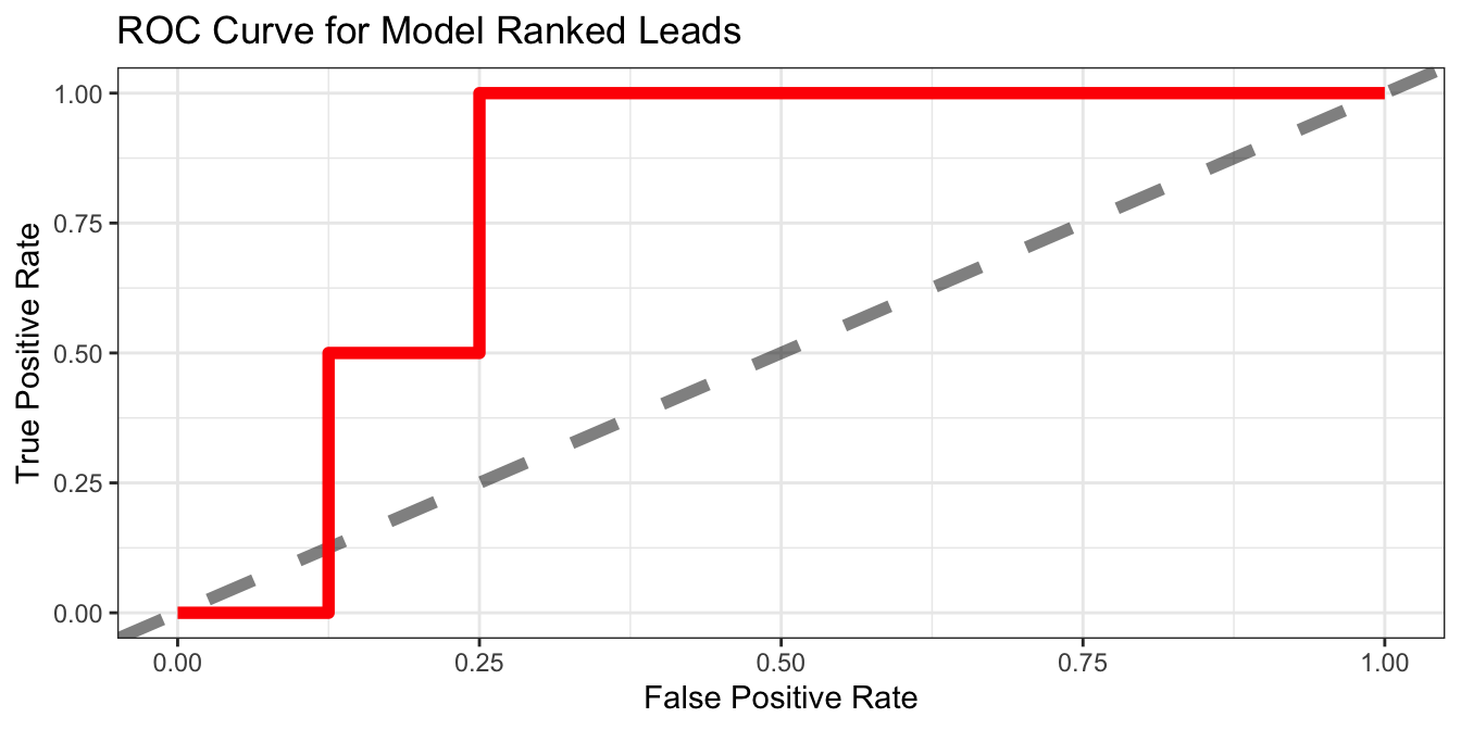
For reference, the point (0.25, 1.0) means that our model exhausted 25% of the bad leads in order to identify 100% of the good leads. This curve is called the Receiver Operating Characteristic (ROC curve). Measuring area under the ROC curve gives an indication of how well the leads are ranked. A perfect model will have AUC ROC = 1, and a random guess model should have AUC ROC = 0.5.
One last bit about our objective – It doesn’t matter how well we rank the weakest leads because we only have the resources to call the top leads. For this reason, partial AUC ROC would be even better objective function, but since it’s a little more complex we’ll stick to maximizing AUC ROC.
The Models
I built three models to solve this problem. Each model has some benefits and drawbacks which I’ll discuss, but I’m not going to display their results. This would be counterproductive for a few reasons
- There’s not enough data to make confident model comparisons
- I made up the data
- I didn’t spend a lot of time tuning each model’s hyper parameters
Instead, think of this as a starter kit/guide to solving your own problem.
Logistic Regression
This is probably the purist model of three with the strongest statistical foundation. It can work really well, but it’ll quickly fall apart when important assumptions are violated (as they often are when working with real world data).
Pros
– Can work extremely well (if the data is very clean and satisfies a bunch of nice properties)
– Fast
– Simple. You could build it in an Excel spreadsheet
Cons
– Requires imputation for missing values
– Poorly handles non monotonic relationships and spikes (e.g. imputing -1 for NA values where all other values are $ \geq 0 $)
– Requires one-hot-encoding for unordered categorical features
– Can be difficult to measure variable importance
– R implementation doesn’t directly provide a regularization term
Implementations
Random Forest
This is probably my favorite solution. It’s easy to set up and it almost always works. Plus it’s pretty darn cool.
Pros
– Almost always performs well
– Easy to understand the model’s logic
– Can handle complex interactions of multiple variables
– Does a good job of modeling non monotonic relationships and spikes in the data
– Easy to measure the importance of each predictor
– Easy to tune the model’s hyper parameters
Cons
– Can be difficult to explain exactly why a certain prediction was made on test data
– Can be difficult to diagnose issues
– Requires imputation for missing values
– Scikit-Learn requires one-hot-encoding for unordered categorical features which leads to problems with performance and possible speed issues
– R implementation only allows categorical features with up to 53 unique categories
Implementations
Gradient Boosting (XGBoost)
In terms of performance, this one’s probably the best. XGBoost wins something like half of all Kaggle competitions. However, it’s fairly complex, can be difficult to tune, and it’s predictions are even more mystical than random forest.
Pros
– Usually performs extremely well
– Very fast
– Smart handling of missing values
– Easy to measure variable importance
Cons
– Can be difficult to explain exactly why a certain prediction was made on test data
– Difficult to prepare dataset for model training and predictions
– Difficult to tune hyper parameters
– Requires one-hot encoding categorical features