Decision Trees in R using rpart
R’s rpart package provides a powerful framework for growing classification and regression trees. To see how it works, let’s get started with a minimal example.
Motivating Problem
First let’s define a problem. There’s a common scam amongst motorists whereby a person will slam on his breaks in heavy traffic with the intention of being rear-ended. The person will then file an insurance claim for personal injury and damage to his vehicle, alleging that the other driver was at fault. Suppose we want to predict which of an insurance company’s claims are fraudulent using a decision tree.
To start, we need to build a training set of known fraudulent claims.
train <- data.frame(
  ClaimID = c(1,2,3),
  RearEnd = c(TRUE, FALSE, TRUE),
  Fraud = c(TRUE, FALSE, TRUE)
)

train
##   ClaimID RearEnd Fraud
## 1       1    TRUE  TRUE
## 2       2   FALSE FALSE
## 3       3    TRUE  TRUE
First Steps with rpart
In order to grow our decision tree, we have to first load the rpart package. Then we can use the rpart() function, specifying the model formula, data, and method parameters. In this case, we want to classify the feature Fraud using the predictor RearEnd, so our call to rpart() should look like
library(rpart)

mytree <- rpart(
  Fraud ~ RearEnd,
  data = train,
  method = "class"
)

mytree
## n= 3
##
## node), split, n, loss, yval, (yprob)
##       * denotes terminal node
##
## 1) root 3 1 TRUE (0.3333333 0.6666667) *
Notice the output shows only a root node. This is because rpart has some default parameters that prevented our tree from growing. Namely minsplit and minbucket. minsplit is “the minimum number of observations that must exist in a node in order for a split to be attempted” and minbucket is “the minimum number of observations in any terminal node”. See what happens when we override these parameters.
mytree <- rpart(
  Fraud ~ RearEnd,
  data = train,
  method = "class",
  minsplit = 2,
  minbucket = 1
)

mytree
## n= 3
##
## node), split, n, loss, yval, (yprob)
##       * denotes terminal node
##
## 1) root 3 1 TRUE (0.3333333 0.6666667)
##   2) RearEnd< 0.5 1 0 FALSE (1.0000000 0.0000000) *
##   3) RearEnd>=0.5 2 0 TRUE (0.0000000 1.0000000) *
Now our tree has a root node, one split and two leaves (terminal nodes). Observe that rpart encoded our boolean variable as an integer (false = 0, true = 1). We can plot mytree by loading the rattle package (and some helper packages) and using the fancyRpartPlot() function.
library(rattle)
library(rpart.plot)
library(RColorBrewer)

# plot mytree
fancyRpartPlot(mytree, caption = NULL)
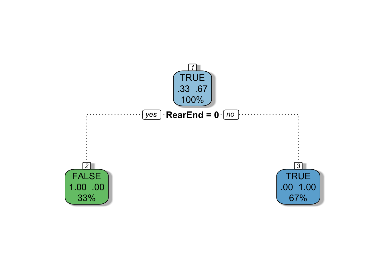
The decision tree correctly identified that if a claim involved a rear-end collision, the claim was most likely fraudulent.
By default, rpart uses gini impurity to select splits when performing classification. (If you’re unfamiliar read this article.) You can use information gain instead by specifying it in the parms parameter.
mytree <- rpart(
  Fraud ~ RearEnd,
  data = train,
  method = "class",
  parms = list(split = 'information'),
  minsplit = 2,
  minbucket = 1
)

mytree
## n= 3
##
## node), split, n, loss, yval, (yprob)
##       * denotes terminal node
##
## 1) root 3 1 TRUE (0.3333333 0.6666667)
##   2) RearEnd< 0.5 1 0 FALSE (1.0000000 0.0000000) *
##   3) RearEnd>=0.5 2 0 TRUE (0.0000000 1.0000000) *
Now suppose our training set looked like this..
train <- data.frame(
  ClaimID = c(1,2,3),
  RearEnd = c(TRUE, FALSE, TRUE),
  Fraud = c(TRUE, FALSE, FALSE)
)

train
##   ClaimID RearEnd Fraud
## 1       1    TRUE  TRUE
## 2       2   FALSE FALSE
## 3       3    TRUE FALSE
If we try to build a decision tree on this data..
mytree <- rpart(
  Fraud ~ RearEnd,
  data = train,
  method = "class",
  minsplit = 2,
  minbucket = 1
)

mytree
## n= 3
##
## node), split, n, loss, yval, (yprob)
##       * denotes terminal node
##
## 1) root 3 1 FALSE (0.6666667 0.3333333) *
Once again we’re left with just a root node. Internally, rpart keeps track of something called the complexity of a tree. The complexity measure is a combination of the size of a tree and the ability of the tree to separate the classes of the target variable. If the next best split in growing a tree does not reduce the tree’s overall complexity by a certain amount, rpart will terminate the growing process. This amount is specified by the complexity parameter, cp, in the call to rpart(). Setting cp to a negative amount ensures that the tree will be fully grown.
mytree <- rpart(
  Fraud ~ RearEnd,
  data = train,
  method = "class",
  minsplit = 2,
  minbucket = 1,
  cp = -1
)

fancyRpartPlot(mytree, caption = NULL)
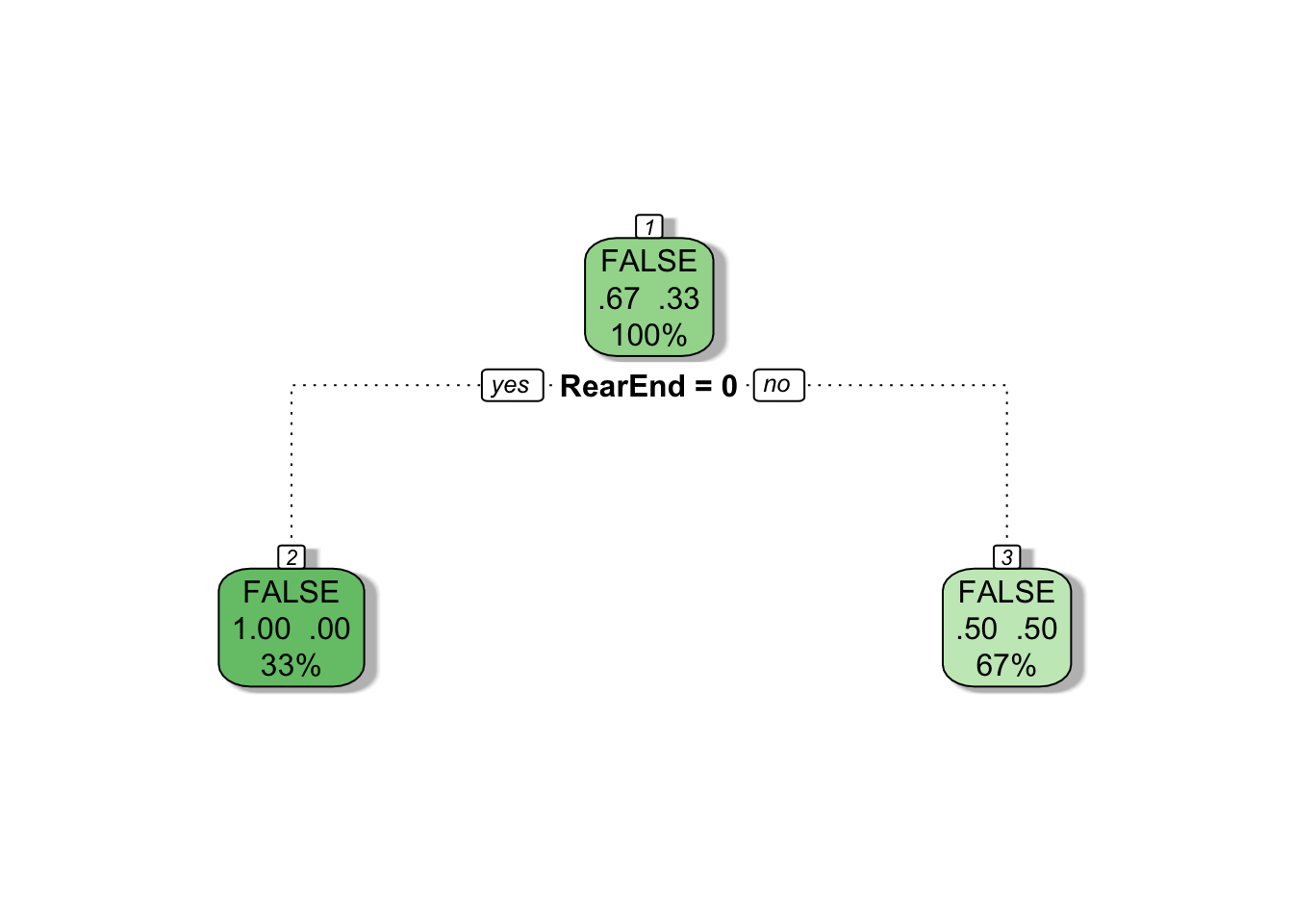
This is not always a good idea since it will typically produce over-fitted trees, but trees can be pruned back as discussed later in this article.
You can also weight each observation for the tree’s construction by specifying the weights argument to rpart().
mytree <- rpart(
  Fraud ~ RearEnd,
  data = train,
  method = "class",
  minsplit = 2,
  minbucket = 1,
  weights = c(0.4, 0.4, 0.2)
)

fancyRpartPlot(mytree, caption = NULL)
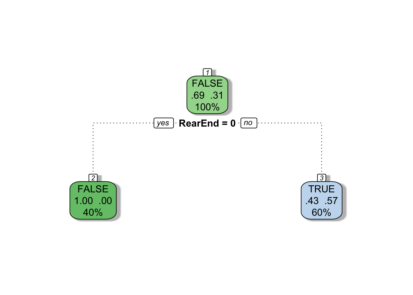
One of the best ways to identify a fraudulent claim is to hire a private investigator to monitor the activities of a claimant. Since private investigators don’t work for free, the insurance company will have to strategically decide which claims to investigate. To do this, they can use a decision tree model based off some initial features of the claim. If the insurance company wants to aggressively investigate claims (i.e. investigate a lot of claims), they can train their decision tree in a manner that will penalize incorrectly labeled fraudulent claims more than it penalizes incorrectly labeled non-fraudulent claims.
To alter the default, equal penalization of mislabeled target classes set the loss component of the parms parameter to a matrix where the (i,j) element is the penalty for misclassifying an i as a j. (The loss matrix must have 0s in the diagonal). For example, consider the following training data.
train <- data.frame(
  ClaimID = 1:7,
  RearEnd = c(TRUE, TRUE, FALSE, FALSE, FALSE, FALSE, FALSE),
  Whiplash = c(TRUE, TRUE, TRUE, TRUE, TRUE, FALSE, FALSE),
  Fraud = c(TRUE, TRUE, TRUE, FALSE, FALSE, FALSE, FALSE)
)

train
##   ClaimID RearEnd Whiplash Fraud
## 1       1    TRUE     TRUE  TRUE
## 2       2    TRUE     TRUE  TRUE
## 3       3   FALSE     TRUE  TRUE
## 4       4   FALSE     TRUE FALSE
## 5       5   FALSE     TRUE FALSE
## 6       6   FALSE    FALSE FALSE
## 7       7   FALSE    FALSE FALSE
Now let’s grow our decision tree, restricting it to one split by setting the maxdepth argument to 1.
mytree <- rpart(
  Fraud ~ RearEnd + Whiplash,
  data = train,
  method = "class",
  maxdepth = 1,
  minsplit = 2,
  minbucket = 1
)

fancyRpartPlot(mytree, caption = NULL)
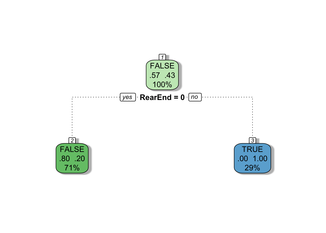
rpart has determined that RearEnd was the best variable for identifying a fraudulent claim. BUT there was one fraudulent claim in the training dataset that was not a rear-end collision. If the insurance company wants to identify a high percentage of fraudulent claims without worrying too much about investigating non-fraudulent claims they can set the loss matrix to penalize claims incorrectly labeled as fraudulent three times less than claims incorrectly labeled as non-fraudulent.
lossmatrix <- matrix(c(0,1,3,0), byrow = TRUE, nrow = 2)
lossmatrix
##      [,1] [,2]
## [1,]    0    1
## [2,]    3    0

mytree <- rpart(
  Fraud ~ RearEnd + Whiplash,
  data = train,
  method = "class",
  maxdepth = 1,
  minsplit = 2,
  minbucket = 1,
  parms = list(loss = lossmatrix)
)

fancyRpartPlot(mytree, caption = NULL)
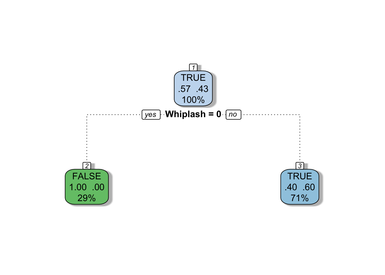
Now our model suggests that Whiplash is the best variable to identify fraudulent claims. What I just described is known as a valuation metric and its up to the discretion of the insurance company to decide on it. Yaser Abu-Mostafa of Caltech has a great talk on this topic.
Now let’s see how rpart interacts with factor variables. Suppose the insurance company hires an investigator to assess the activity level of claimants. Activity levels can be very active, active, inactive, or very inactive.
Dataset 1
train <- data.frame(
ClaimID = c(1,2,3,4,5),
Activity = factor(
x = c("active", "very active", "very active", "inactive", "very inactive"),
levels = c("very inactive", "inactive", "active", "very active")
),
Fraud = c(FALSE, TRUE, TRUE, FALSE, TRUE)
)
train
## ClaimID Activity Fraud
## 1 1 active FALSE
## 2 2 very active TRUE
## 3 3 very active TRUE
## 4 4 inactive FALSE
## 5 5 very inactive TRUE
mytree <- rpart(
Fraud ~ Activity,
data = train,
method = "class",
minsplit = 2,
minbucket = 1
)
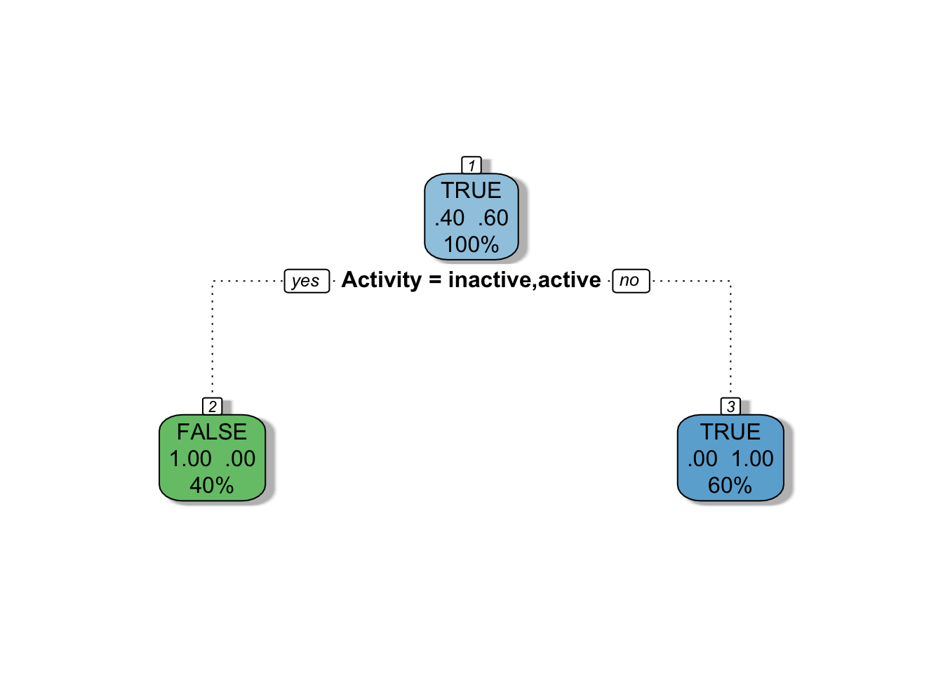
fancyRpartPlot(mytree, caption = NULL)
Dataset 2
train <- data.frame(
ClaimID = 1:5,
Activity = factor(
x = c("active", "very active", "very active", "inactive", "very inactive"),
levels = c("very inactive", "inactive", "active", "very active"),
ordered = TRUE
),
Fraud = c(FALSE, TRUE, TRUE, FALSE, TRUE)
)
train
## ClaimID Activity Fraud
## 1 1 active FALSE
## 2 2 very active TRUE
## 3 3 very active TRUE
## 4 4 inactive FALSE
## 5 5 very inactive TRUE
mytree <- rpart(
Fraud ~ Activity,
data = train,
method = "class",
minsplit = 2,
minbucket = 1
)
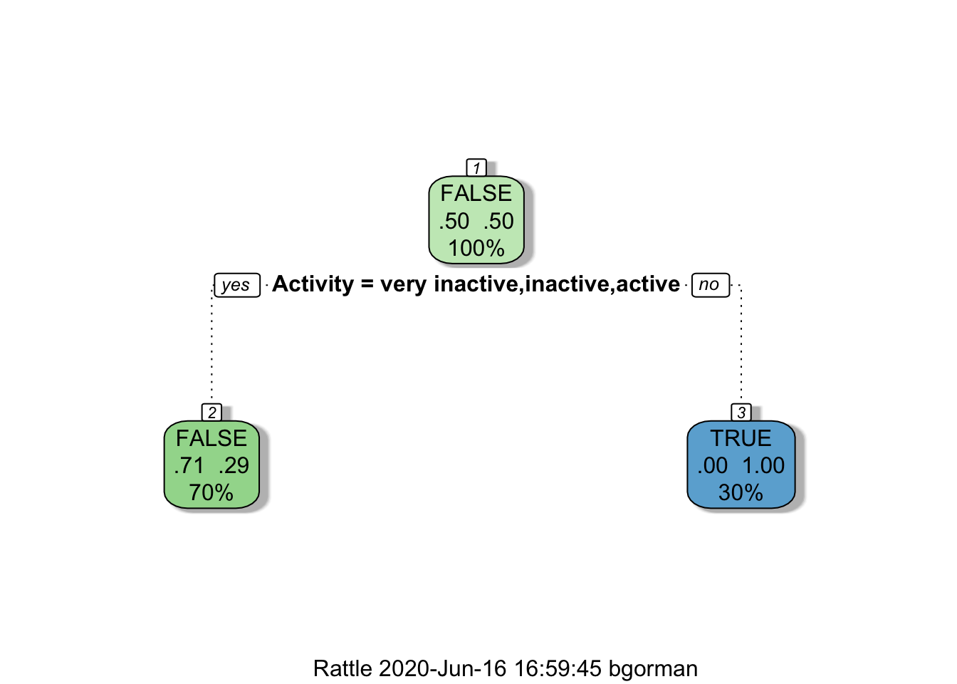
fancyRpartPlot(mytree, caption = NULL)
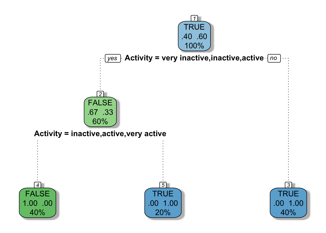
In the first dataset, we did not specify that Activity was an ordered factor, so rpart tested every possible way to split the levels of the Activity vector. In the second dataset, Activity was specified as an ordered factor so rpart only tested splits that separated the ordered set of Activity levels. (For more explanation of this, see this post and/or this post.)
It’s usually a good idea to prune a decision tree. Fully grown trees don’t perform well against data not in the training set because they tend to be over-fitted so pruning is used to reduce their complexity by keeping only the most important splits.
train <- data.frame(
ClaimID = 1:10,
RearEnd = c(TRUE, TRUE, TRUE, FALSE, FALSE, FALSE, FALSE, TRUE, TRUE, FALSE),
Whiplash = c(TRUE, TRUE, TRUE, TRUE, TRUE, FALSE, FALSE, FALSE, FALSE, TRUE),
Activity = factor(
x = c("active", "very active", "very active", "inactive", "very inactive", "inactive", "very inactive", "active", "active", "very active"),
levels = c("very inactive", "inactive", "active", "very active"),
ordered=TRUE
),
Fraud = c(FALSE, TRUE, TRUE, FALSE, FALSE, TRUE, TRUE, FALSE, FALSE, TRUE)
)
train
## ClaimID RearEnd Whiplash Activity Fraud
## 1 1 TRUE TRUE active FALSE
## 2 2 TRUE TRUE very active TRUE
## 3 3 TRUE TRUE very active TRUE
## 4 4 FALSE TRUE inactive FALSE
## 5 5 FALSE TRUE very inactive FALSE
## 6 6 FALSE FALSE inactive TRUE
## 7 7 FALSE FALSE very inactive TRUE
## 8 8 TRUE FALSE active FALSE
## 9 9 TRUE FALSE active FALSE
## 10 10 FALSE TRUE very active TRUE
# Grow a full tree
mytree <- rpart(
Fraud ~ RearEnd + Whiplash + Activity,
data = train,
method = "class",
minsplit = 2,
minbucket = 1,
cp = -1
)
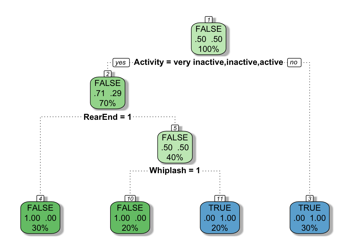
fancyRpartPlot(mytree, caption = NULL)
You can view the importance of each variable in the model by referencing the variable.importance attribute of the resulting rpart object. From the rpart documentation, “An overall measure of variable importance is the sum of the goodness of split measures for each split for which it was the primary variable…”
mytree$variable.importance
##  Activity  Whiplash   RearEnd
## 3.0000000 2.0000000 0.8571429
When rpart grows a tree it performs 10-fold cross validation on the data. Use printcp() to see the cross validation results.
printcp(mytree)
##
## Classification tree:
## rpart(formula = Fraud ~ RearEnd + Whiplash + Activity, data = train,
##     method = "class", minsplit = 2, minbucket = 1, cp = -1)
##
## Variables actually used in tree construction:
## [1] Activity RearEnd  Whiplash
##
## Root node error: 5/10 = 0.5
##
## n= 10
##
##     CP nsplit rel error xerror    xstd
## 1  0.6      0       1.0    2.0 0.00000
## 2  0.2      1       0.4    0.4 0.25298
## 3 -1.0      3       0.0    0.4 0.25298
The rel error of each iteration of the tree is the fraction of mislabeled elements in the iteration relative to the fraction of mislabeled elements in the root. In this example, 50% of training cases are fraudulent. The first splitting criteria is “Is the claimant very active?”, which separates the data into a set of three cases, all of which are fraudulent and a set of seven cases of which two are fraudulent. Labeling the cases at this point would produce an error rate of 20% which is 40% of the root node error rate (i.e. it’s 60% better). The cross validation error rates and standard deviations are displayed in the columns xerror and xstd respectively.
As a rule of thumb, it’s best to prune a decision tree using the cp of smallest tree that is within one standard deviation of the tree with the smallest xerror. In this example, the best xerror is 0.4 with standard deviation 0.25298. So, we want the smallest tree with xerror less than 0.65298. This is the tree with cp = 0.2, so we’ll want to prune our tree with a cp slightly greater than than 0.2.
mytree <- prune(mytree, cp = 0.21)
fancyRpartPlot(mytree)
From here we can use our decision tree to predict fraudulent claims on an unseen dataset using the predict() function.
test <- data.frame(
  ClaimID = 1:10,
  RearEnd = c(FALSE, TRUE, TRUE, FALSE, FALSE, FALSE, FALSE, TRUE, TRUE, FALSE),
  Whiplash = c(FALSE, TRUE, TRUE, TRUE, TRUE, FALSE, FALSE, FALSE, FALSE, TRUE),
  Activity = factor(
    x = c("inactive", "very active", "very active", "inactive", "very inactive", "inactive", "very inactive", "active", "active", "very active"),
    levels = c("very inactive", "inactive", "active", "very active"),
    ordered = TRUE
  )
)

test
##    ClaimID RearEnd Whiplash      Activity
## 1        1   FALSE    FALSE      inactive
## 2        2    TRUE     TRUE   very active
## 3        3    TRUE     TRUE   very active
## 4        4   FALSE     TRUE      inactive
## 5        5   FALSE     TRUE very inactive
## 6        6   FALSE    FALSE      inactive
## 7        7   FALSE    FALSE very inactive
## 8        8    TRUE    FALSE        active
## 9        9    TRUE    FALSE        active
## 10      10   FALSE     TRUE   very active

# Predict the outcome and the possible outcome probabilities
test$FraudClass <- predict(mytree, newdata = test, type = "class")
test$FraudProb <- predict(mytree, newdata = test, type = "prob")
test
##    ClaimID RearEnd Whiplash      Activity FraudClass FraudProb.FALSE
## 1        1   FALSE    FALSE      inactive      FALSE       0.7142857
## 2        2    TRUE     TRUE   very active       TRUE       0.0000000
## 3        3    TRUE     TRUE   very active       TRUE       0.0000000
## 4        4   FALSE     TRUE      inactive      FALSE       0.7142857
## 5        5   FALSE     TRUE very inactive      FALSE       0.7142857
## 6        6   FALSE    FALSE      inactive      FALSE       0.7142857
## 7        7   FALSE    FALSE very inactive      FALSE       0.7142857
## 8        8    TRUE    FALSE        active      FALSE       0.7142857
## 9        9    TRUE    FALSE        active      FALSE       0.7142857
## 10      10   FALSE     TRUE   very active       TRUE       0.0000000
##    FraudProb.TRUE
## 1       0.2857143
## 2       1.0000000
## 3       1.0000000
## 4       0.2857143
## 5       0.2857143
## 6       0.2857143
## 7       0.2857143
## 8       0.2857143
## 9       0.2857143
## 10      1.0000000
In summary, the rpart package is pretty sweet. I tried to cover the most important features of the package, but I suggest you read through the rpart vignette to understand the things I skipped. Also, I’d like to point out that a single decision tree usually won’t have much predictive power but an ensemble of varied decision trees such as random forests and boosted models can perform extremely well.