Logistic Regression Fundamentals
Logistic regression is a generalized linear model most commonly used for classifying binary data. It’s output is a continuous range of values between 0 and 1 (commonly representing the probability of some event occurring), and its input can be a multitude of real-valued and discrete predictors.
Motivating Problem
Suppose you want to predict the probability someone is a homeowner based solely on their age. You might have a dataset like
| Age | HomeOwner |
|---|---|
| 13 | FALSE |
| 13 | FALSE |
| 15 | FALSE |
| ... | ... |
| 74 | TRUE |
| 75 | TRUE |
| 79 | TRUE |
As with any binary variable, it makes sense to code TRUE values as 1s and FALSE values as 0s. Then you can plot the data. Our homeowner dataset looks like this
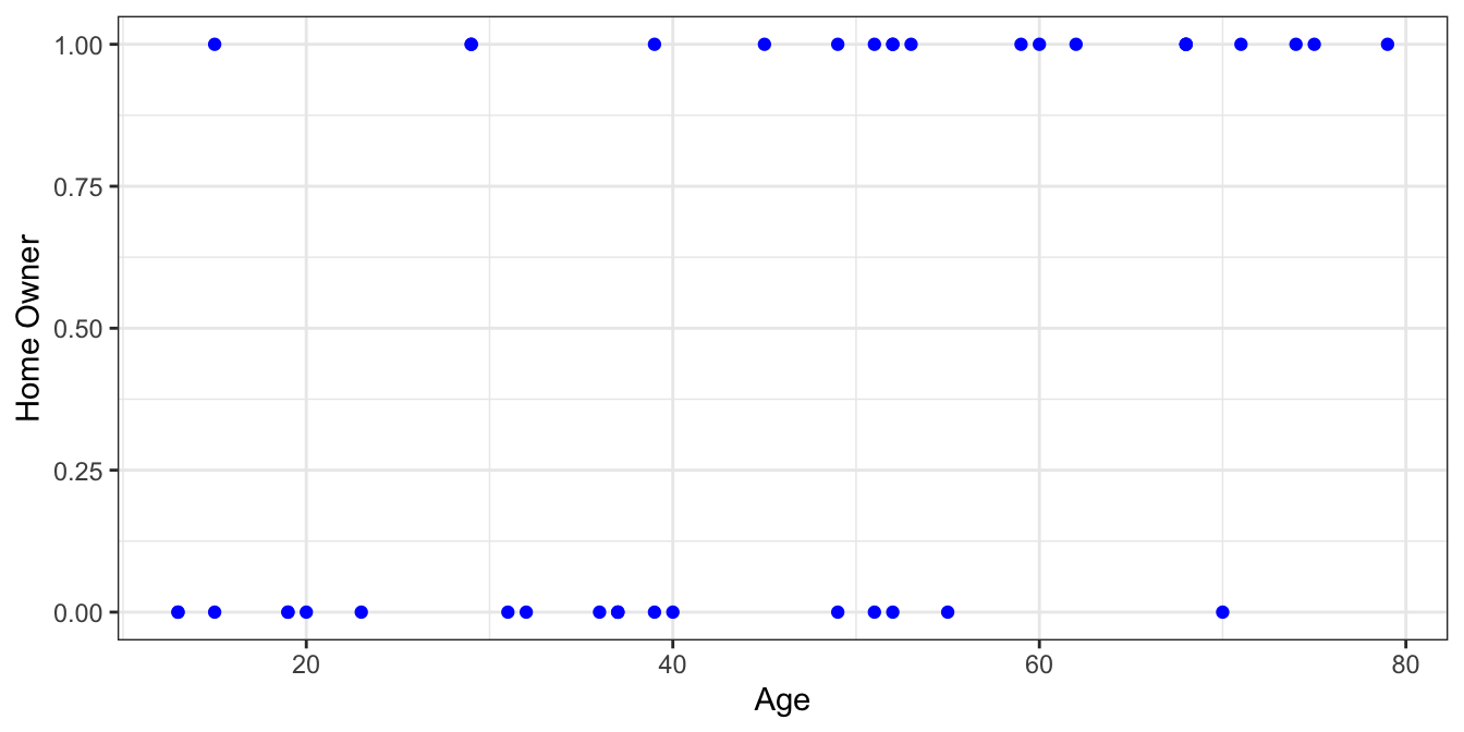
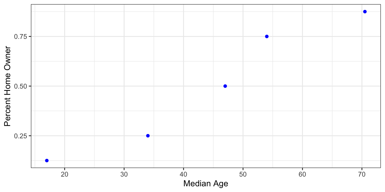
There’s definitely more positive samples as age increases which makes sense. If we decide to group the data into equal size bins we can calculate the proportion of positive samples for each group.
| Bin | Samples | MedianAge | PctHomeOwner |
|---|---|---|---|
| [10, 24) | 8 | 17.0 | 0.125 |
| [24, 38) | 8 | 34.0 | 0.250 |
| [38, 52) | 8 | 47.0 | 0.500 |
| [52, 66) | 8 | 54.0 | 0.750 |
| [66, 80] | 8 | 70.5 | 0.875 |
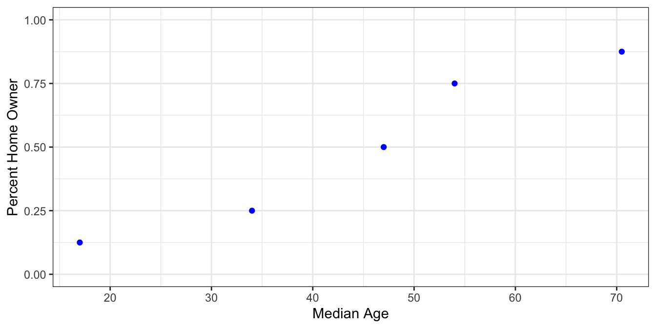
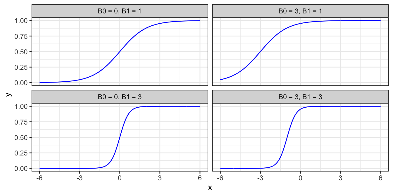
Notice the data starting to take an S shape. This is a common and natural occurrence for a variety of random processes, particularly where the explanatory variable and the response variable have a monotonic relationship. One such S-shaped function is the logistic function.
$$ \sigma(t) = \frac{1}{1+e^{-t}} $$
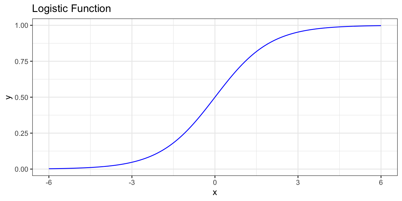
Writing $ t $ as $ B_0 + B_1 $ lets us change the horizontal position of the curve by varying $ B_0 $ and the steepness of the curve by varying $ B_1 $.
$$ F(x) = \frac {1}{1+e^{-(\beta_0 + \beta_1 x)}} $$
Fitting a model to the data
At this point we’d like to fit a logistic curve to our data. There are two distinct ways to do this depending on the type of data to be fitted.
Method 1
First we’ll look at fitting a logistic curve to binned, or grouped data. For example, suppose we didn’t have individual Yes/No responses of whether someone was a homeowner, but instead had an aggregated data set like
| MedianAge | PctHomeOwner |
|---|---|
| 17.0 | 0.125 |
| 34.0 | 0.250 |
| 47.0 | 0.500 |
| 54.0 | 0.750 |
| 70.5 | 0.875 |
Recall our last form of the logistic function
$ F(x) = \frac {1}{1+e^{-(\beta_0 + \beta_1 x)}} $
where we interpret $ F(x) $ to be the probability that someone is a homeowner. We can rearrange this equation as follows
$ \ln (\frac{F(x)}{1 - F(x)}) = \beta_0 + \beta_1 x $
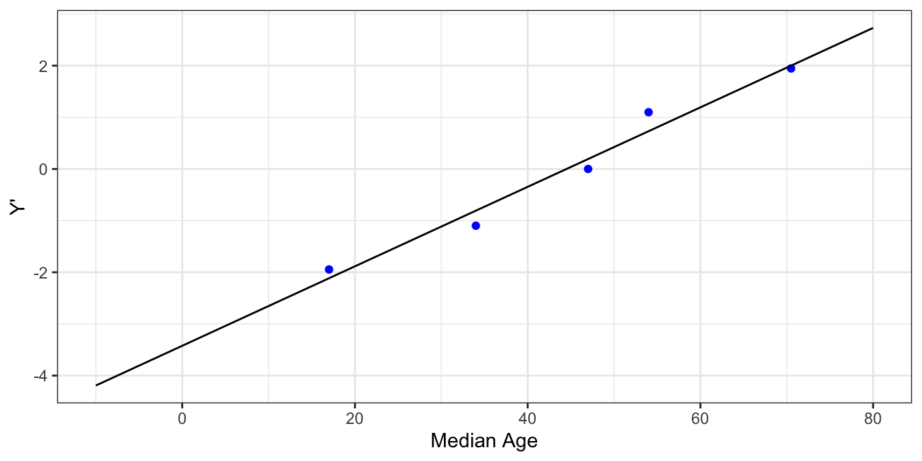
Notice that the modified function is linear in terms of $ x $. So, if we take our sample data and create a transformed column $ Y' $ equal to $ \ln(\frac{PcntHomeowner}{1-PcntHomeowner}) $ then we can fit $ Y' = B_0 + B_1x $ using ordinary least squares.
| MedianAge | PctHomeOwner | Y' |
|---|---|---|
| 17.0 | 0.125 | -1.945910 |
| 34.0 | 0.250 | -1.098612 |
| 47.0 | 0.500 | 0.000000 |
| 54.0 | 0.750 | 1.098612 |
| 70.5 | 0.875 | 1.945910 |
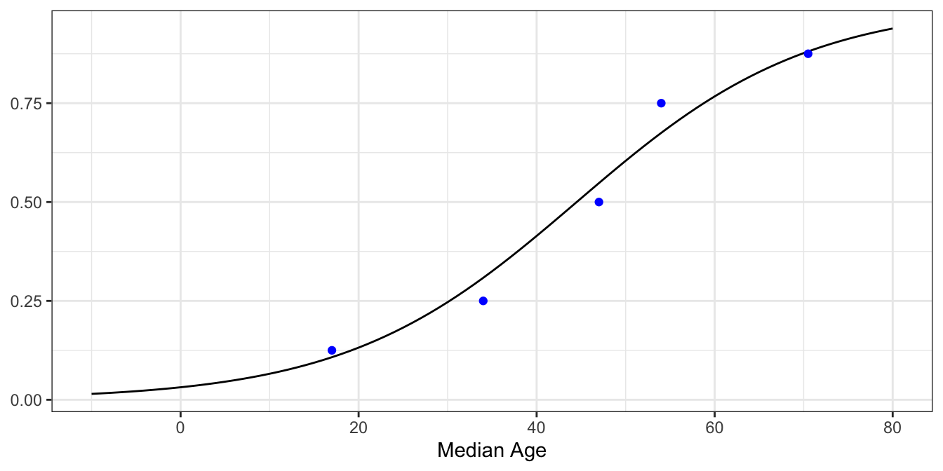
From here we can transform the fitted linear model to a logistic model. We have
$ Y' = \ln (\frac{F(x)}{1 - F(x)}) = \beta_0 + \beta_1x \Rightarrow F(x) = \frac{1}{1+e^{-(\beta_0 + \beta_1x)}} $
(Nothing special here - just the logistic function.)
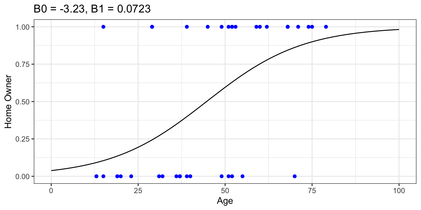
Finally, plotting the model against our data..
Before we wrap up method 1, let’s take another look at our linear model
$ \ln (\frac{F(x)}{1 - F(x)}) = \beta_0 + \beta_1 x $
First of all, this is the inverse of the logistic function. Secondly, notice the $ \frac{F}{(1-F)} $ part. Remember, $ F $ is the probability of success. So, $ \frac{F}{(1-F)} $ is the odds of success.
The odds of something happening is the probability of it happening divided by the probability of it not happening. If the probability of a horse winning the Kentucky Derby is 0.2, then the odds of that horse winning are 0.2/0.8 = 0.25 (or more commonly stated, the odds of the horse losing are 4 or “4 to 1”).
Recapping, for some probability of success $ p $, the odds of success are $ \frac{p}{1-p} $ and the log-odds are $ ln(\frac{p}{1-p}) $. The function $ ln(\frac{p}{1-p}) $ is special enough to warrant its own name - the logit function. Notice it’s equivalent to the linear model we fit, $ ln(\frac{F}{1-F}) = B_0 + B_1x $. In other words, we fit a logistic regression to our data by fitting a linear model to the log-odds of our sample data.
Method 2
In Method 1 we were able to use linear regression to fit our data because our dataset had probabilities of homeownership. On the other hand, if our data just has {0, 1} response values we’ll have to use a more sophisticated technique - maximum likelihood estimation.
First, recall the Bernoulli distribution. A Bernoulli random variable X is just a binary random variable (0 or 1) with probability of success p. (I.e. P(X=1) = p). Thus the Bernoulli distribution is defined by a single parameter, $ p $. Furthermore, its expected value equals $ p $.
Next, let’s take another look at our plotted data.

Now pick an x value, say 50, and imagine slicing the data in a small neighborhood around 50.
| Age | HomeOwner |
|---|---|
| 49 | 0 |
| 49 | 1 |
| 51 | 1 |
| 51 | 0 |
Looking at the data we find 2 positive and 2 negative samples. In this case we can think of each response variable near $ Age = 50 $ as a random variable from some Bernoulli distribution whose $ p $ value is somewhere in the neighborhood of 0.5.
Now let’s slice the data in the neighborhood of 70.
| Age | HomeOwner |
|---|---|
| 68 | 1 |
| 68 | 1 |
| 68 | 1 |
| 70 | 0 |
| 71 | 1 |
We can think of these samples as random variables sampled from some other Bernoulli distribution which have a $ p $ value close to 0.80. This coincides with our intuition that the probability of someone being a homeowner generally increases with their age.
Generalizing this idea, we can assume that at each point $ x $ the samples close to $ x $ follow a Bernoulli distribution whose expected value is some function of $ x $. We’ll call that function $ p(x) $. Since we want to model our data with the logistic function
$ F(x) = \frac {1}{1+e^{-(\beta_0 + \beta_1 x)}} $,
we can treat $ F(x) $ and $ p(x) $ to be the same. In other words, we can think of our logistic function as defining an infinite set of Bernoulli distributions.
Now suppose we guess some parameters $ B_0 $ and $ B_1 $ which appear to fit the data well, say $ B_0 = -3.5 $ and $ B_1 = 0.06 $.
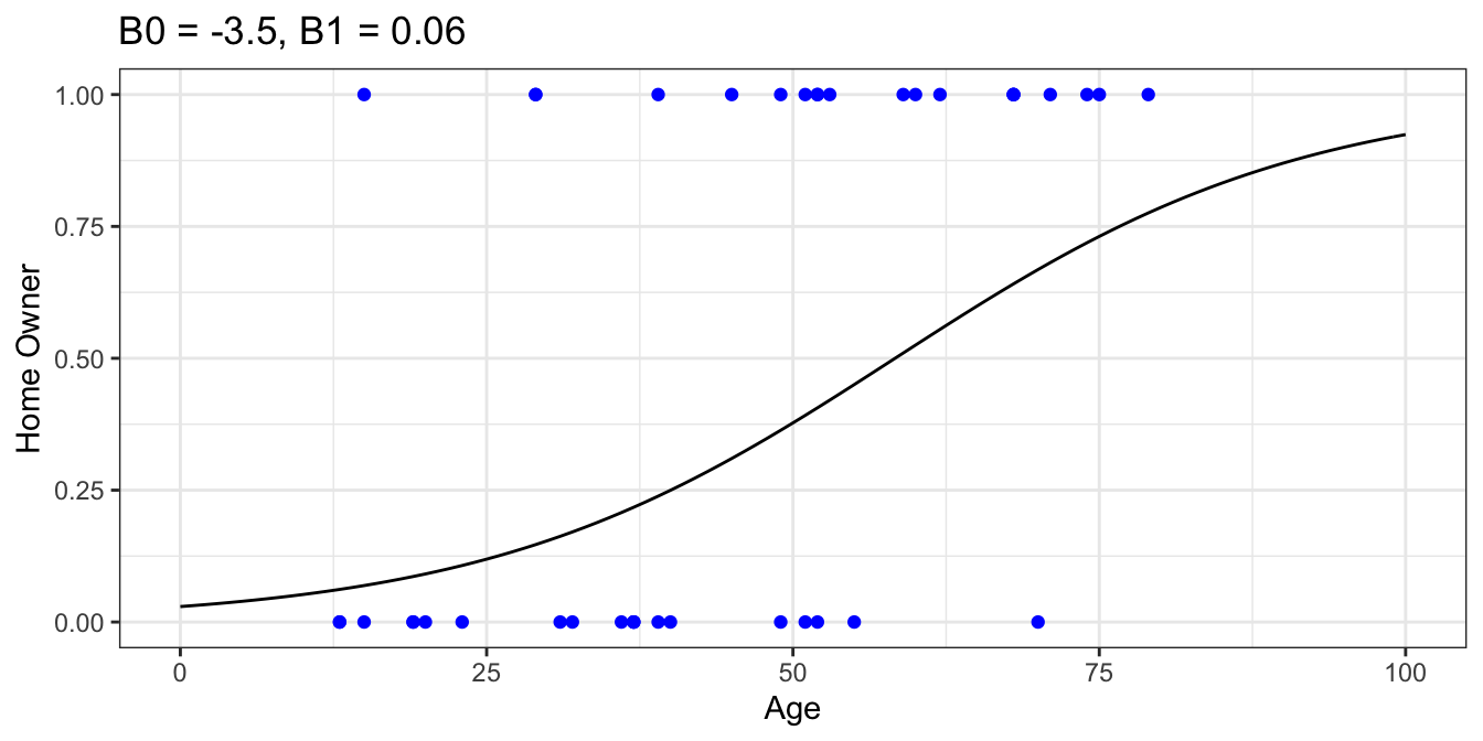
Assuming our guessed model is the true model for whether or not someone is a homeowner based on their age, what is the probability of our sampled data occurring? In other words, what is the probability that a random 13-year-old isn’t a homeowner AND another random 13-year-old isn’t a homeowner … AND a random 75-year-old is a homeowner AND a random 79-year-old is a homeowner?
According to our model, the probability that a random 13-year-old isn’t a homeowner is $ p(Y = 0 \mid x = 13) = 1 - F(13) = 0.93 $. The probability that a random 75-year-old is a homeowner is $ F(75) = 0.73 $, etc. If we assume each of these instances are independent, then the probability of all of them occurring is $ (1-F(13)) \cdot (1-F(13)) \cdots F(75) \cdot F(79) $.
What we just described is calculating the probability or “likelihood” of our samples having their response values according to our model $ F(x, B_0 = -3.5, B_1 = 0.06) $. For a set of samples assumed to be from some logistic regression model, we can define the likelihood of the specific model with parameters $ B_0 $ and $ B_1 $ as
$$ \begin{aligned} \mathcal{L}(B0, B1; \boldsymbol{samples}) &= \prod_{i=1}^n P[Y_i=y_i \mid p_i=F(x_i, B0, B1)] \\ &= \prod_{i=1}^n F(x_i, B0, B1)^{y_i}(1-F(x_i, B0, B1))^{(1-y_i)} \end{aligned} $$
where $ (x_i, y_i) $ is the ith observation in our sample data.
Plugging in $ F $ gives
$$ \mathcal{L}(B0, B1; \boldsymbol{samples}) = \prod_{i=1}^n (\frac {1}{1+e^{-(\beta_0 + \beta_1 x_i)}})^{y_i}(1-\frac {1}{1+e^{-(\beta_0 + \beta_1 x_i)}})^{(1-y_i)} $$
This is called the likelihood function. The parameters ($ B_0 $, $ B_1 $) that yield the largest value of $ L $ are exactly the parameters we want to use for our logistic regression model. The process of finding those optimum parameters is called maximum likelihood estimation.
With that said, maximum likelihood estimation is a deep topic and probably warrants its own separate article. For that reason, I’ll leave out the gritty details. Fortunately for the practitioners out there, a number of maximum likelihood estimation methods have been implemented in open-source statistical libraries. Using scikit-learn with our sample data yields $ B_0 = -3.23 $ and $ B_1 = 0.0723 $.