R – Introduction to Factors Tutorial

A factor variable (commonly called a categorical variable outside of R) is a variable that takes on a limited set of values. For example, a vector that stores days of the week {Sunday, Monday, etc.} or colors from the set {Red, Blue, Green} should be encoded as a factor. By contrast, a vector of person names {Bill, Sue, Jane, …} should generally be designated as a character vector since there is an unlimited set of possible names a person can take. Let’s make this more clear with some examples..

First we create a vector of colors.

colors <- c("blue", "red", "green")
class(colors)
## [1] "character"

By default, R creates a character vector. We can use the factor() function to explicitly create a vector of factors.

colors <- factor(c("blue", "red", "green"))
class(colors)
## [1] "factor"

Notice the output when we print the colors vector.

colors
## [1] blue  red   green
## Levels: blue green red

R displays our vector of colors with something additional – Levels.

The levels of a factor are the possible values that the variable can take. By default, when you create a factor vector, R sets the levels of the factor to be the unique set of values inside the vector, and R orders the levels alphabetically.

Suppose you’re a teacher and you give your students a survey to evaluate your performance. One of your evaluation criteria might be “Your teacher had strong knowledge of the subject” with possible answers {Strongly Agree, Agree, Disagree, Strongly Disagree}. Suppose the student responses were {Agree, Agree, Strongly Agree, Disagree, Agree}. We can create a vector of these responses by

responses <- factor(c("Agree", "Agree", "Strongly Agree", "Disagree", "Agree"))
responses
## [1] Agree          Agree          Strongly Agree Disagree       Agree         
## Levels: Agree Disagree Strongly Agree

Luckily for you, none of the students strongly disagreed with the statement. However, since it was an option in the survey it should be included in the levels attribute of the factor. You can correct this by explicitly setting the levels parameter in the call to factor().

responses <- factor(
  x = c("Agree", "Agree", "Strongly Agree", "Disagree", "Agree"),
  levels = c("Strongly Agree", "Agree", "Disagree", "Strongly Disagree")
)
responses
## [1] Agree          Agree          Strongly Agree Disagree       Agree         
## Levels: Strongly Agree Agree Disagree Strongly Disagree

Now, with the extra information provided in the levels attribute we can do things like plot a bar graph of the students’ responses including responses that were not selected.

Using ggplot2…

library(ggplot2)

# Create a data frame for call to ggplot()
df <- data.frame(responses = responses)

# Plot
ggplot(data = df, aes(x = responses)) + 
  geom_bar() + 
  scale_x_discrete(drop = FALSE)

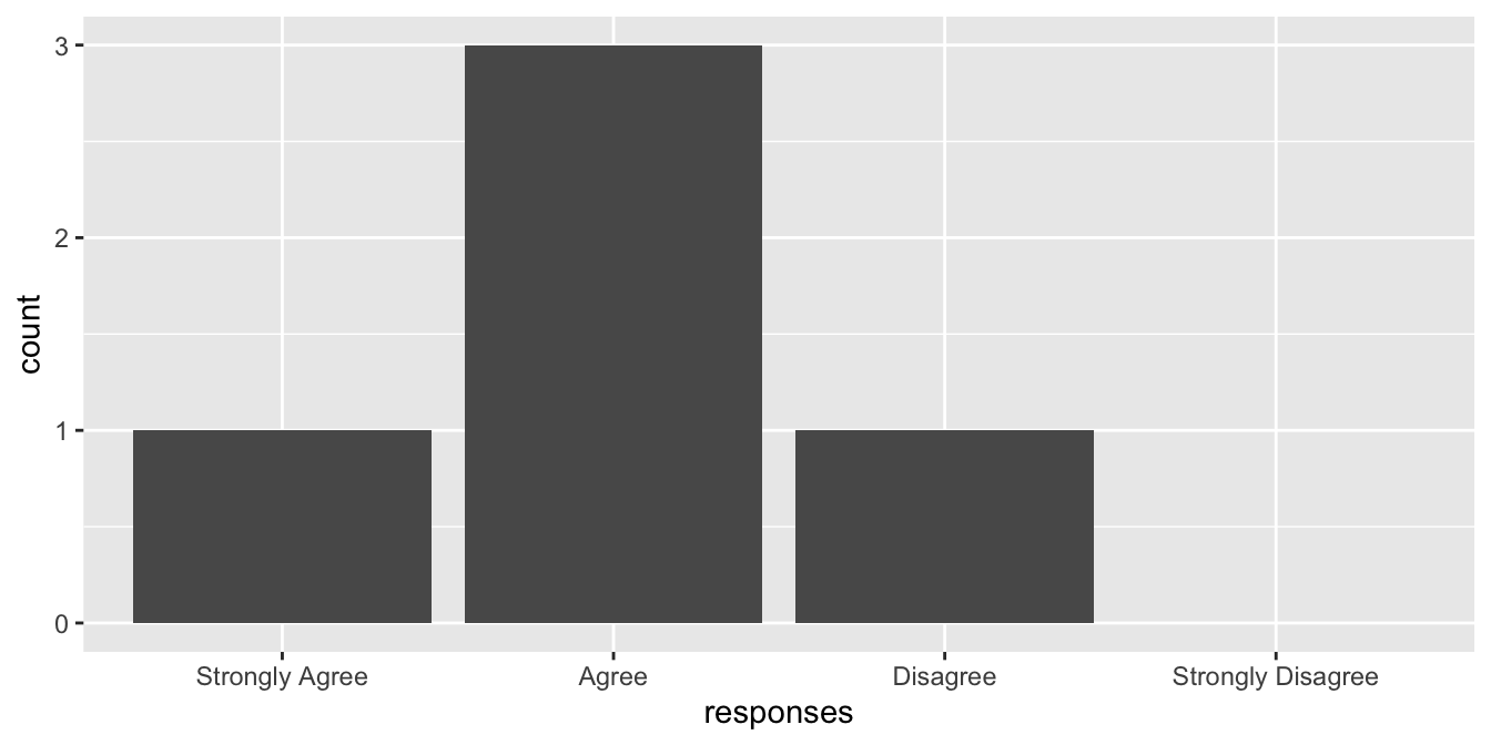
Here, drop = FALSE tells the plot not to drop unused levels (i.e. include Strongly Disagree on the x axis).

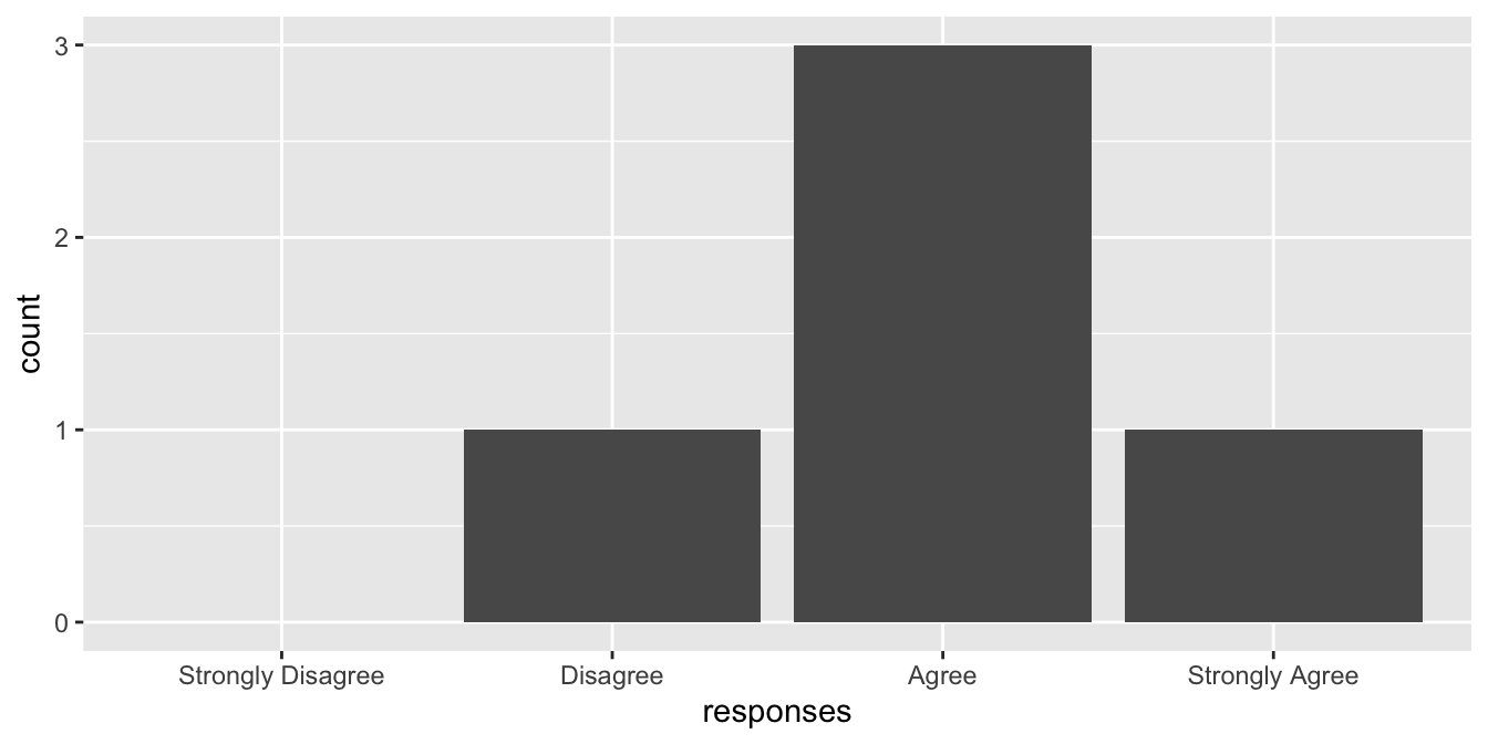
Also note that plots will display the values of a factor in the order of the levels of the factor. In the above example, since we explicitly defined the levels attribute as c(“Strongly Agree”, “Agree”, “Disagree”, “Strongly Disagree”), our bar plot displayed the bars in that order. We can plot the response options in the reverse order by resetting the levels of the responses vector.

responses <- factor(
  x = responses,
  levels = c("Strongly Disagree", "Disagree", "Agree", "Strongly Agree")
)
df <- data.frame(responses = responses)
ggplot(data = df, aes(x = responses)) + geom_bar() + scale_x_discrete(drop = FALSE)

There’s an important distinction to make between the two examples of factors we discusses above. Responses {Strongly Agree, Agree, Disagree, Strongly Disagree} have an inherent order whereas colors {red, blue, green} do not. To see whether a factor is ordered, use the is.ordered() function.

colors <- factor(c("blue", "red", "green"))
is.ordered(colors)
## [1] FALSE

responses <- factor(
  x = c("Agree", "Agree", "Strongly Agree", "Disagree", "Agree"),
  levels = c("Strongly Agree", "Agree", "Disagree", "Strongly Disagree")
)
is.ordered(responses)
## [1] FALSE

Factors are not “ordered” by default. We can use the ordered parameter of the factor() function to tell R that a factor has inherent order.

responses <- factor(
  x = c("Agree", "Agree", "Strongly Agree", "Disagree", "Agree"),
  levels = c("Strongly Agree", "Agree", "Disagree", "Strongly Disagree"),
  ordered = TRUE
)
is.ordered(responses)
## [1] TRUE

Printing the responses vector gives

responses
## [1] Agree          Agree          Strongly Agree Disagree       Agree         
## Levels: Strongly Agree < Agree < Disagree < Strongly Disagree

Notice the levels are printed with “<“s indicating that they have a meaningful order. Certain probabilistic models such as decision trees will take this into account. For example, consider a model that uses the responses of your student survey to try to predict whether a student failed your class. If you feed the responses to the model as an unordered factor, the model might consider all possible combinations of responses to predict whether a student failed

{Agree, Strongly Disagree} vs {Strongly Agree, Disagree}
{Strongly Agree, Disagree, Strongly Disagree} vs {Agree}
…
{Strongly Disagree} vs {Strongly Agree, Agree, Disagree}

If you feed the responses to the model as an ordered factor, the model may only look at the following combinations of responses

{Strongly Agree, Agree, Disagree} vs {Strongly Disagree}
{Strongly Agree, Agree} vs {Disagree, Strongly Disagree}
{Strongly Agree} vs {Agree, Disagree, Strongly Disagree}

The latter approach being much more reasonable for your classification model.